A R package to compare two random variables and determine which of them takes lower values.
All the details and the methodology are available in our paper [1]. In the following, we show a quick start example. Let us see how to use this package to compare the scores of two optimization algorithms PL-EDA and PL-GS [2] in the instance N-t70n11xx of the Linear Ordering Problem [3]. Suppose that we are given 400 measurements of the objective functions (from now on score) of these two algorithms in this instance.
We just save the fitness values in two arrays:
Click here to expand code
PL_EDA_fitness <- c(
52235, 52485, 52542, 52556, 52558, 52520, 52508, 52491, 52474, 52524,
52414, 52428, 52413, 52457, 52437, 52449, 52534, 52531, 52476, 52434,
52492, 52554, 52520, 52500, 52342, 52520, 52392, 52478, 52422, 52469,
52421, 52386, 52373, 52230, 52504, 52445, 52378, 52554, 52475, 52528,
52508, 52222, 52416, 52492, 52538, 52192, 52416, 52213, 52478, 52496,
52444, 52524, 52501, 52495, 52415, 52151, 52440, 52390, 52428, 52438,
52475, 52177, 52512, 52530, 52493, 52424, 52201, 52484, 52389, 52334,
52548, 52560, 52536, 52467, 52392, 51327, 52506, 52473, 52087, 52502,
52533, 52523, 52485, 52535, 52502, 52577, 52508, 52463, 52530, 52507,
52472, 52400, 52511, 52528, 52532, 52526, 52421, 52442, 52532, 52505,
52531, 52644, 52513, 52507, 52444, 52471, 52474, 52426, 52526, 52564,
52512, 52521, 52533, 52511, 52416, 52414, 52425, 52457, 52522, 52508,
52481, 52439, 52402, 52442, 52512, 52377, 52412, 52432, 52506, 52524,
52488, 52494, 52531, 52471, 52616, 52482, 52499, 52386, 52492, 52484,
52537, 52517, 52536, 52449, 52439, 52410, 52417, 52402, 52406, 52217,
52484, 52418, 52550, 52513, 52530, 51667, 52185, 52089, 51853, 52511,
52051, 52584, 52475, 52447, 52390, 52506, 52514, 52452, 52526, 52502,
52422, 52411, 52171, 52437, 52323, 52488, 52546, 52505, 52563, 52457,
52502, 52503, 52126, 52537, 52435, 52419, 52300, 52481, 52419, 52540,
52566, 52547, 52476, 52448, 52474, 52438, 52430, 52363, 52484, 52455,
52420, 52385, 52152, 52505, 52457, 52473, 52503, 52507, 52429, 52513,
52433, 52538, 52416, 52479, 52501, 52485, 52429, 52395, 52503, 52195,
52380, 52487, 52498, 52421, 52137, 52493, 52403, 52511, 52409, 52479,
52400, 52498, 52482, 52440, 52541, 52499, 52476, 52485, 52294, 52408,
52426, 52464, 52535, 52512, 52516, 52531, 52449, 52507, 52485, 52491,
52499, 52414, 52403, 52398, 52548, 52536, 52410, 52549, 52454, 52534,
52468, 52483, 52239, 52502, 52525, 52328, 52467, 52217, 52543, 52391,
52524, 52474, 52509, 52496, 52432, 52532, 52493, 52503, 52508, 52422,
52459, 52477, 52521, 52515, 52469, 52416, 52249, 52537, 52494, 52393,
52057, 52513, 52452, 52458, 52518, 52520, 52524, 52531, 52439, 52530,
52422, 52649, 52481, 52256, 52428, 52425, 52458, 52488, 52502, 52373,
52426, 52441, 52471, 52468, 52465, 52265, 52455, 52501, 52340, 52457,
52275, 52527, 52574, 52474, 52487, 52416, 52634, 52514, 52184, 52430,
52462, 52392, 52529, 52178, 52495, 52438, 52539, 52430, 52459, 52312,
52437, 52637, 52511, 52563, 52270, 52341, 52436, 52515, 52480, 52569,
52490, 52453, 52422, 52443, 52419, 52512, 52447, 52425, 52509, 52180,
52521, 52566, 52060, 52425, 52480, 52454, 52501, 52536, 52143, 52432,
52451, 52548, 52508, 52561, 52515, 52502, 52468, 52373, 52511, 52516,
52195, 52499, 52534, 52453, 52449, 52431, 52473, 52553, 52444, 52459,
52536, 52413, 52537, 52537, 52501, 52425, 52507, 52525, 52452, 52499
)
PL_GS_fitness <- c(
52476, 52211, 52493, 52484, 52499, 52500, 52476, 52483, 52431, 52483,
52515, 52493, 52490, 52464, 52478, 52440, 52482, 52498, 52460, 52219,
52444, 52479, 52498, 52481, 52490, 52470, 52498, 52521, 52452, 52494,
52451, 52429, 52248, 52525, 52513, 52489, 52448, 52157, 52449, 52447,
52476, 52535, 52464, 52453, 52493, 52438, 52489, 52462, 52219, 52223,
52514, 52476, 52495, 52496, 52502, 52538, 52491, 52457, 52471, 52531,
52488, 52441, 52467, 52483, 52476, 52494, 52485, 52507, 52224, 52464,
52503, 52495, 52518, 52490, 52508, 52505, 52214, 52506, 52507, 52207,
52531, 52492, 52515, 52497, 52476, 52490, 52436, 52495, 52437, 52494,
52513, 52483, 52522, 52496, 52196, 52525, 52490, 52506, 52498, 52250,
52524, 52469, 52497, 52519, 52437, 52481, 52237, 52436, 52508, 52518,
52490, 52501, 52508, 52476, 52520, 52435, 52463, 52481, 52486, 52489,
52482, 52496, 52499, 52443, 52497, 52464, 52514, 52476, 52498, 52496,
52498, 52530, 52203, 52482, 52441, 52493, 52532, 52518, 52474, 52498,
52512, 52226, 52538, 52477, 52508, 52243, 52533, 52463, 52440, 52246,
52209, 52488, 52530, 52195, 52487, 52494, 52508, 52505, 52444, 52515,
52499, 52428, 52498, 52244, 52520, 52463, 52187, 52484, 52517, 52504,
52511, 52530, 52519, 52514, 52532, 52203, 52485, 52439, 52496, 52443,
52503, 52520, 52516, 52478, 52473, 52505, 52480, 52196, 52492, 52527,
52490, 52493, 52252, 52470, 52493, 52533, 52506, 52496, 52519, 52492,
52509, 52530, 52213, 52499, 52492, 52528, 52499, 52526, 52521, 52488,
52485, 52502, 52515, 52470, 52207, 52494, 52527, 52442, 52200, 52485,
52489, 52499, 52488, 52486, 52232, 52477, 52485, 52490, 52524, 52470,
52504, 52501, 52497, 52489, 52152, 52527, 52487, 52501, 52504, 52494,
52484, 52213, 52449, 52490, 52525, 52476, 52540, 52463, 52200, 52471,
52479, 52504, 52526, 52533, 52473, 52475, 52518, 52507, 52500, 52499,
52512, 52478, 52523, 52453, 52488, 52523, 52240, 52505, 52532, 52504,
52444, 52194, 52514, 52474, 52473, 52526, 52437, 52536, 52491, 52523,
52529, 52535, 52453, 52522, 52519, 52446, 52500, 52490, 52459, 52467,
52456, 52490, 52521, 52484, 52508, 52451, 52231, 52488, 52485, 52215,
52493, 52475, 52474, 52508, 52524, 52477, 52514, 52452, 52491, 52473,
52441, 52520, 52471, 52466, 52475, 52439, 52483, 52491, 52204, 52500,
52488, 52489, 52519, 52495, 52448, 52453, 52466, 52462, 52489, 52471,
52484, 52483, 52501, 52486, 52494, 52473, 52481, 52502, 52516, 52223,
52490, 52447, 52222, 52469, 52509, 52194, 52490, 52484, 52446, 52487,
52476, 52509, 52496, 52459, 52474, 52501, 52516, 52223, 52487, 52468,
52534, 52522, 52474, 52227, 52450, 52506, 52193, 52429, 52496, 52493,
52493, 52488, 52190, 52509, 52434, 52469, 52510, 52481, 52520, 52504,
52230, 52500, 52487, 52517, 52473, 52488, 52450, 52203, 52215, 52490,
52479, 52515, 52210, 52485, 52516, 52504, 52521, 52499, 52503, 52526)The first step is to visualize the data with a simple visualization tool such as a box-plot or a histogram.
boxplot(x = list("PL_EDA_fitness"=PL_EDA_fitness, "PL_GS_fitness"=PL_GS_fitness))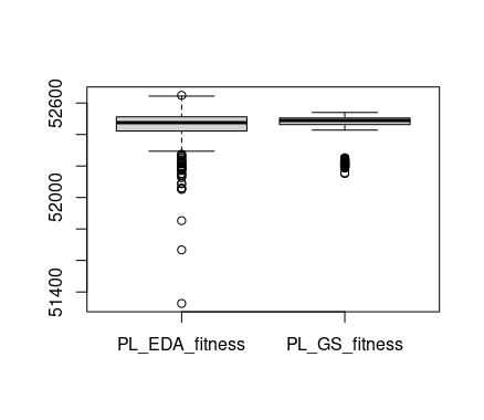
Unfortunately, in this case, the box-plot does not show a result that can be used to compare the two algorithms. In part, this is due to their similarity in performance but it is also because of the large amount of outliers. This is the kind of situation in which the cumulative difference-plot can help.
The Linear Ordering Problem is a maximization problem, therefore we need isMinimizationProblem=FALSE. The cumulative difference-plot needs to know if it is a maximization or a minimization problem, because the best values are compared in the left side of the plot, while the worst are compared at the right side of the plot. With the code below, we can generate the cumulative difference-plot. By default, the confidence level of the confidence band is 95%.
library("RVCompare")
cumulative_difference_plot(X_A_observed=PL_EDA_fitness,
                            X_B_observed=PL_GS_fitness,
                            isMinimizationProblem=FALSE,
                            labelA="PL-EDA",
                            labelB="PL-GS")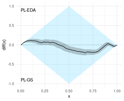
The cumulative difference-plot compares the best scores on the left side (x < 0.5) and the worst scores in the right side (x > 0.5). In addition, when the difference is positive, then it means that PL-EDA is better than PL-GS in that quantile (see the labels in the plot). For example, since the difference is positive in x = 0.25, we can say that PL-EDA has a better 25% quantile than PL-GS. We can deduce many things from this plot. In the following, we interpret the estimation of the cumulative difference plot, but take into account that the actual difference is likely differnt to the estimation and is somewhere inside the confidence band.
-
A.- The probability that a score of PL-EDA is better than a score of PL-GS is a little higher than 0.5.
To deduce this probability from the graph, we compute the difference between the area on top of diff(x)=0 and the area under diff(x)=0, and we add 0.5 to this difference. In this example, the estimated probability that the score of PL-EDA is better than the score of PL-GS is (A1 - A2 + A3 - A4) + 0.5.

-
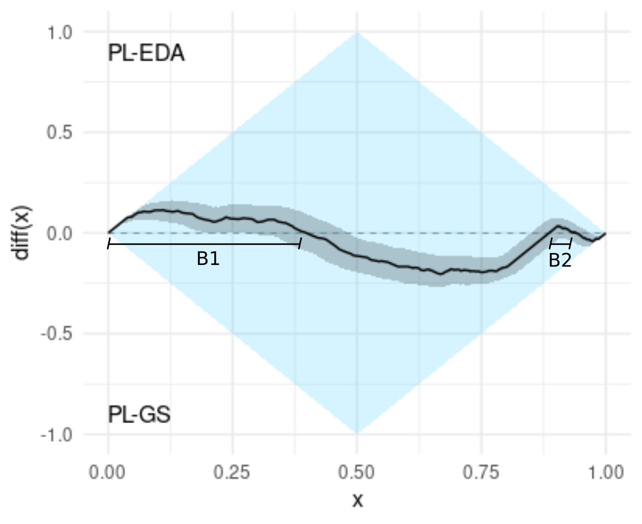
B.- Neither algorithm dominates the other one, and what is more, the dominance rate is near 0.5
The dominance rate can be deduced from the graph by measuring the poportion in which the difference is positive. In this example, the dominance rate is B1 + B2. The dominance rate can be interpreted as the extent to which PL-EDA dominates PL-GS (see [1] for details).
-
C.- The difference is positive when x < 0.3, and therefore, if we only consider the best 30% values of both algorithms, PL-EDA dominates PL-GS
We say that one algorithm dominates the other one when the cumulative distribution function of one of the scores is higher or equal than the otherone in all the domain of definintion, see [1] for details. This is known as first order stochastic dominance [4].
-
D.- Similarly, the difference is negative when x > 0.98. In this case, we conclude that if we only consider the worst 2% values of PL-EDA and PL-GS, then PL-GS dominates PL-EDA.
Note that these 2% worse values are much less likely than the best 30% values.
-
E.- Similarly, the difference is negative when x > 0.98. In this case, we conclude that if we only consider the worst 2% values of PL-EDA and PL-GS, then PL-GS dominates PL-EDA.
The difference is negative at x = 0.5 and at x = 0.75. This can be interpreted as PL-GS having a better median and a better 75% quantile.
Summarizing the above points, we conclude that the performance of the algorithms is quite similar, and PL-EDA can obtain both better and worse scores than PL-GS. The probability that PL-EDA takes these better values is much higher than the probability that it takes worse values. Therefore, if we are in a setting in which repeating the execution of the algorithms is reasonable, PL-EDA is a much better algorithm. On the other hand, if it is critical to avoid really bad values, then PL-GS would be preferred.
If you found this work useful, I would appreciate a citation.
@article{doi:10.1080/10618600.2022.2084405,
author = {Etor Arza and Josu Ceberio and Ekhiñe Irurozki and Aritz Pérez},
title = {Comparing two samples through stochastic dominance: a graphical approach},
journal = {Journal of Computational and Graphical Statistics},
volume = {0},
number = {ja},
pages = {1-38},
year  = {2022},
publisher = {Taylor & Francis},
doi = {10.1080/10618600.2022.2084405},
URL = {https://doi.org/10.1080/10618600.2022.2084405},
eprint = {https://doi.org/10.1080/10618600.2022.2084405}
}[1] Arza, E., Ceberio, J., Irurozki, E., & Pérez, A. (2022). Comparing two samples through stochastic dominance: A graphical approach. Journal of Computational and Graphical Statistics, 1–38. https://doi.org/10.1080/10618600.2022.2084405. Open version: https://doi.org/10.48550/arXiv.2203.07889.
[2] Santucci, V., Ceberio, J., & Baioletti, M. (2020). Gradient search in the space of permutations: An application for the linear ordering problem. Proceedings of the 2020 Genetic and Evolutionary Computation Conference Companion, 1704-1711. https://doi.org/10.1145/3377929.3398094
[3] Schiavinotto, T., & Stützle, T. (2004). The Linear Ordering Problem: Instances, Search Space Analysis and Algorithms. Journal of Mathematical Modelling and Algorithms, 3(4), 367-402. https://doi.org/10.1023/B:JMMA.0000049426.06305.d8
[4] Quirk, J. P., & Saposnik, R. (1962). Admissibility and measurable utility functions. The Review of Economic Studies, 29(2), 140-146. https://doi.org/10.2307/2295819