Please note the current accepted version of the krill stock assessment is https://github.com/ccamlr/Grym_Base_Case/tree/Simulations
The idea of this repository is to provide a base case implementation of the Grym assessment for E. superba. The base cases will be performed using the same basic configuration as the assessments evaluated in during the 2010 WG-EMM that were fitted using the GYM software with the following changes:
- they will be fitted in using the Grym package in R,
- they will be area specific,
- they will use updated biological parameters for each Subarea where they are available.
The idea for having a base case is to essentially have assessments that are ready for management advice using previously agreed upon configurations available for WG-EMM-2021. They will provide the infrastructure for other implementations to be explored (such as RecMaker recruitment, different recruitment functions etc.) whilst still having assessments for each Subarea ready to go should these different implementations not be ready in time for WG-EMM-2021.
A short video describing how the Grym will be used to determine sustainable yield is available here.
If you have not done so yet, download and install R (https://cloud.r-project.org/) and Rstudio (https://rstudio.com/products/rstudio/download/#download). If you already have, make sure these are up to date.
Start R studio. In the Console, type:
install.packages(c("remotes","devtools","knitr","ggplot2","dplyr","tidyr","furrr","rmarkdown","future"))
In the Console, type:
remotes::install_github("AustralianAntarcticDivision/Grym", build_vignettes=TRUE)
In the Console, type:
library(Grym)
then,
browseVignettes(package="Grym")
This will open a web browser from which you can access a description of the Grym as well as an example (“Icefish”). It is recommended to view these documents as HTML pages.
Additional examples are located inside the Grym package directory. To find its location in your computer, type:
find.package("Grym")
You may then go to that location in your computer (outside of R Studio), and in the ‘examples’ subfolder, you will find the "Examples.html" file which contains further useful documentation.
You may also be interested in particular functions used within the Grym; to access help files for functions, type in the Console (for example, for the function project()):
?project
If you wish to see the source code of a function, type:
View(project)
In addition to the documents and tutorials mentioned above, the following video tutorials are available:
Video 1: https://youtu.be/JPWauYbmzB0
Title: Grym (R implementation of the Generalized Yield Model) tutorial 1.
Description: Principals of the model, how cohorts move through time and age. Presented by Simon Wotherspoon (UTAS).
Video 2: https://youtu.be/AnLEUxyCwB8
Title: Grym (R implementation of the Generalized Yield Model) tutorial 2.
Description: The ‘Krill 1996’ example, structure of the code. Presented by Simon Wotherspoon (UTAS).
Video 3: https://youtu.be/2TT15v-9oNw
Title: Grym (R implementation of the Generalized Yield Model) tutorial 3.
Description: The ‘Krill 1996’ example, step by step execution. Presented by Simon Wotherspoon (UTAS).
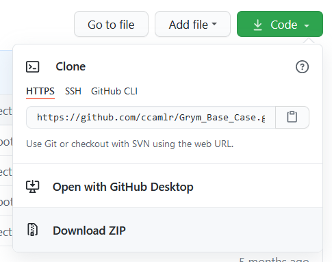
At the top of this page, go to ‘Code’ and ‘download ZIP’:
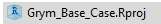
Extract the contents of that zip file on your computer. In the resulting folder you will find an R project file named ‘Grym_Base_Case.Rproj’:
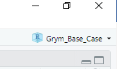
Double click on that file. You are now inside the “Grym_Base_Case” R project, as shown by the icon at the top right corner of R Studio:
Whenever you wish to use the scripts contained in this repository, it is crucial to first open the R project file named “Grym_Base_Case.Rproj”. This will ensure that R Studio knows where all the files are.
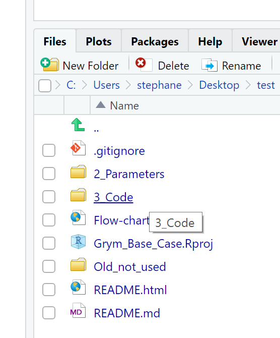
Once inside the project, you may now run some simulations. Go to the file browser inside R studio and click on "3_Code":
The code is embedded in an Rmarkdown file named “48.1_base_case.rmd”. Click on it, it will open inside R studio. Prior to running your first test, it is recommended to do a simulation with few runs otherwise it might take a long time. Inside the markdown, navigate to the line where the number of runs is set:
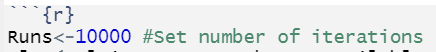
And change to Runs<-100, for example. Then save.
To execute the code, you must ‘knit’ the markdown, by clicking on the knit button:
Once the knitting process is finished, the result is shown in a pop-up window (48.1_base_case.html).
Because the repository will change over time, you must keep your version, on your computer, up to date. To update your repository, Simply re-download it as per Section 4 instructions.
The code is designed to work in two tiers, at the bottom is the core functions use to produce the assessment for example: Projection_function.R,prfit.r, above this sits the three Rmarkdown documents 1_Setup_48.1.rmd, 2_Generate_recruitment.rmd and 3_Projection_48.1.rmd. The idea being for each scenario you create a copy of the 1_Setup file and have the approporiate scenario parameters. If you are using new recruitment values or your time steps/age classes change you run the 2_Generate_recruitment file giving it the list from the setup file. Finally you run the 3_Projection file to actually run the simulation.
The reason for this structure is:
-
The .R files in the Source folder don't change for example the
Projection_function.Rcontains theKrillProjection()function that will be used for each run of the Grym and has no hard coded or default biological parameter values. -
For each scenario you create a copy of the markdown documents and explain how that scenario is different.
The folder '2_Parameters' the scenario setup lists as .rds files, and the recruitment series as .rds. These files are written by the 1_Setup and 2_Generate_recruitment markdowns respectively. If the files are used properly than the setup files will have the naming format: Setup_pars_AREA_SCENARIONAME.rds, Similarly the recruitment file will be: Rec_pars_AREA_RMEAN_RSD.rds where the all caps parts are replaced by their respective values.
A note on recruitment; generating recruitment is the slowest part of the assessment that is one of the reasons it is done before the projection, the other being if you want to for example test the difference of changing the length-weight relationship, this method allows you to do that knowing that when you compare the scenarios they are using the exact same recruitment series. You do not need to generate a new recruitment series unless you change any of the following parameters: R.mean, R.sd, R.var, R.Class, R.nsurveys, nsteps or Ages in the setup file from what was used to generate the recruitment series. The function check_params() in the 3_Projection file compares the setup and recruitment parameters to make sure that they match and will return an error if they dont.
- The folder '3_Code' contains the Setup, Recruitment and Projection markdowns with the 'Source' folder containing the functions used in the assessment which shouldn't change.