Census Data
This wiki is an educational guide on how to leverage census data for data analysts/scientists.
The U.S. Census Bureau (USCB) serves as the leading source of quality data about the nation’s people and economy. They measure and disseminate information about the nation’s dynamic economy, society, and institutions, fostering economic growth and advancing scientific understanding, and facilitating informed decisions. Geography plays an important role in all USCB activities by providing the framework used to collect and publish data.
Contents:
- Geographic Entities
- Geographic Identifiers
- Geographic Boundaries (Shapefiles)
- American Community Survey
- Pulling Census Data using USCB APIs
- Data Available in Google BigQuery
- Geocoding Property Addresses
- Urbanization Index (538)
Note: some of this descriptive content is copy/paste from the USCB/other sources and consolidated here in an effort to create a quick learning guide.
The Census Bureau's primary mission is conducting the U.S. census every ten years, which allocates the seats of the U.S. House of Representatives to the states based on their population. The bureau's various censuses and surveys help allocate federal funds every year and it helps states, local communities, and businesses make informed decisions. The information provided by the census informs decisions on where to build and maintain schools, hospitals, transportation infrastructure, and police and fire departments.
In addition to the decennial census, the Census Bureau continually conducts over 130 surveys and programs a year, including the American Community Survey, the U.S. Economic Census, and the Current Population Survey. Furthermore, economic and foreign trade indicators released by the federal government typically contain data produced by the Census Bureau.
The USCB reports data by various geographic units. The top-to-bottom relationship shown below represents containment: the nation contains states, states contain counties, counties contain tracts, tracts contain block groups, and block groups contain blocks. Many other non-nesting reporting units are not shown.
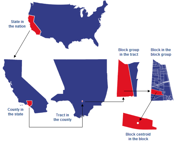
Image Source: ArcGIS
Statistical Entities
-
Census blocks, the smallest geographic area for which the Census Bureau collects and tabulates decennial census data, are formed by streets, roads, railroads, streams and other bodies of water, other visible physical and cultural features, and legal boundaries. These are the building blocks for all geographic boundaries for which the Census Bureau tabulates data. Census blocks generally encompass zero to several hundred people, and are commonly one city block in urban areas.
-
Census Block Groups (BGs) are statistical divisions of census tracts, generally defined to contain between 600 and 3,000 people, and used to present data and control block numbering. A block group consists of clusters of blocks within the same census tract.
-
Census Tracts generally have a population size between 1,200 and 8,000 people, with an optimum size of 4,000 people. A census tract usually covers a contiguous area; however, the spatial size of census tracts varies widely depending on the density of settlement. Census tract boundaries are delineated with the intention of being maintained over a long time so that statistical comparisons could be made from census to census.
Geographic Boundaries
The U.S. Census Bureau conducts the Boundary and Annexation Survey (BAS) annually to collect information about selected legally defined geographic areas. The BAS is used to update information about the legal boundaries and names of all governments. The Census Bureau uses the boundary information collected in the BAS to tabulate data for the decennial and economic censuses, and for annual estimates and surveys such as the American Community Survey (ACS) and the Population Estimates Program (PEP). The Census Bureau provides the results of the BAS to the public as part of the agency’s annual release of TIGER/Line products, including shapefiles.
Understanding the different geographic entities and how they map up to different regions will be important in deciding which level to pull data.
The standard hierarchy of census geographic entities displays the relationships between legal, administrative, and statistical boundaries maintained by the U.S. Census Bureau. The hierarchy provides a quick and easy way to see how the different geographic entities at the Census Bureau relate to one another.
Census blocks are grouped into census block groups, which are grouped into census tracts:

The Census Bureau (and other state and federal agencies) are responsible for assigning geographic identifiers, or GEOIDs, to geographic entities to facilitate the organization, presentation, and exchange of geographic and statistical data.
GEOIDs are numeric codes that uniquely identify all administrative/legal and statistical geographic areas for which the Census Bureau tabulates data. From Alaska, the largest state, to the smallest census block in New York City, every geographic area has a unique GEOID. Some of the most common administrative/legal and statistical geographic entities with unique GEOIDs include states, counties, congressional districts, core based statistical areas (metropolitan and micropolitan areas), census tracts, block groups, and census blocks.
GEOIDs are very important for understanding and interpreting geographic and demographic data and their relationship to one another. Data users rely on GEOIDs to join the appropriate demographic data from censuses and surveys, such as the American Community Survey (ACS), to various levels of geography for data analysis, interpretation, and mapping. Without a common identifier among geographic and demographic datasets, data users would have a difficult time pairing the appropriate demographic data with the appropriate geographic data, thus considerably increasing data processing times and the likelihood of data inaccuracy.
-
Example: census block
The codes used to identify blocks reflect the basic census geographical hierarchy: the country is made up of states, states are made up of counties (and county equivalents like parishes and independent cities), counties are made up of census tracts, and census tracts are made up of census blocks.
A particular census block within the nation must be identified by the following fifteen digits in order:
- States and the territories are identified by a 2-digit code
- Counties within states are identified by a 3-digit code
- Tracts within counties are identified 6-digit code
- Blocks within tracts are identified by a 4-digit code
Census Block 060670011011085:
-
06:California -
067:Sacramento County within California -
001101:Tract 11.01 within Sacramento County -
1085:Block 1085 within Tract 11.01
ZIP Code Tabulation Areas (ZCTAs) are generalized areal representations of United States Postal Service (USPS) ZIP Code service areas. The USPS ZIP Codes identify the individual post office or metropolitan area delivery station associated with mailing addresses. USPS ZIP Codes are not areal features but a collection of mail delivery routes. The term ZCTA was created to differentiate between this entity and true USPS ZIP Codes. ZCTA is a trademark of the U.S. Census Bureau; ZIP Code is a trademark of the U.S. Postal Service.
You should not map ZCTA data directly to ZIP codes.
Note: Google has loaded ZCTA census data into GCP, but named it
zip_cd, but they are ZCTA IDs and shouldn't be joined to zip codes as a first choice.
Because ZIP codes are not 1-1 to ZCTAs, there is a challenge in mapping census data to zip levels. Fortunately, the U.S. Department of Housing and Urban Development's (HUD's) Office of Policy Development and Research (PD&R) created crosswalk files between different census levels to zip codes. These files contain ratios that allow us to separate out portions of population attributes and map them to different zips.
E.g. If a census tract maps to two different zip codes with 90% of addresses mapping to zip a, then we map 90% of the population to zip a. It's not perfect, but it's a much better representation than assuming ZCTAs are 1-1 with ZIP.
-
GCP ZIP to tract cross-reference:
-
GCP Tract to ZIP cross-reference:
For reporting purposes, the U.S. Census Bureau divides the nation into two main types of geographic areas, legal and statistical:
-
Legal Areas:
Defined specifically by law, and include state, local, and tribal government units, and some specially defined administrative areas like congressional districts.
Many, but not all of these areas, are represented by elected officials.
-
Statistical Areas:
Defined directly by the Census Bureau and state, regional, or local authorities for the purpose of presenting data.
The development and maintenance of the statistical entities comprise a significant part of the Census Bureau’s total geographic effort. These statistical areas are designed to have stable boundaries over time; changes are mostly associated with updates from each decennial census.
The Census Bureau cautions against adjusting the boundaries of some statistical units (particularly census tracts and CCDs).
The USCBS TIGER/Line Shapefiles contain geographic extent and boundaries of both legal and statistical entities. This includes boundaries of governmental units that match the data from the surveys that use these geographies.
A shapefile is a geospatial data format for use in geographic information system (GIS) software. Shapefiles spatially describe vector data such as points, lines, and polygons, representing, for instance, landmarks, roads, and lakes. The TIGER/Line Shapefiles are fully supported, core geographic products from the USCB that contain current geography for the United States, the District of Columbia, Puerto Rico, and the Island areas.
Be sure to use the appropriate delineation (2020, 2010, 2000, etc.) when linking to survey data, e.g., 2010 boundaries for 2019 ACS and 2020 boundaries for 2020 ACS.
One of the more useful resources is the American Community Survey conducted annually; results online are generally two years old.
The 2019 ACS data is set to be released between September 2020 and January 2021.
The American Community Survey (ACS) helps local officials, community leaders, and businesses understand the changes taking place in their communities. It is the premier source for detailed population and housing information about our nation. It is an ongoing survey that provides data every year -- giving communities the current information they need to plan investments and services. The ACS covers a broad range of topics about social, economic, demographic, and housing characteristics of the U.S. population.
We'll walk through pulling the 5-year estimates data (instead of 1-year) since multiyear estimates have an increased statistical reliability for less populated areas.
- Usage Guidance
- Public Slack Community: uscensusbureau.slack.com
Available Data:
-
Detailed Tables contain the most detailed cross-tabulations, many of which are published down to block groups. The data are population counts. There are over 20,000 variables in this dataset.
Lowest Level of Geography: Census Block Groups [ex]
-
Subject Tables provide an overview of the estimates available in a particular topic. The data are presented as population counts and percentages. There are over 18,000 variables in this dataset.
Lowest Level of Geography: Census Tracts [ex]
-
Data Profiles contain broad social, economic, housing, and demographic information. The data are presented as population counts and percentages. There are over 1,000 variables in this dataset.
Lowest Level of Geography: Census Tracts [ex]
-
Comparison Profiles are similar to Data Profiles but also include comparisons with past-year data. The current year data are compared with prior 5-Year data and include statistical significance testing. There are over 1,000 variables in this dataset.
Lowest Level of Geography: Places/County Subdivisions [ex]
Boundaries
While geographic boundary changes are not common, they do occur, and those changes can affect a data user’s ability to make comparisons over time. The Census Bureau does not revise ACS data for previous years to reflect changes in geographic boundaries.
In some cases, a geographic boundary may change, but the GEOID may remain the same, so data users need to pay attention to year-to-year changes to make sure the data are comparable over time.
Many statistical areas (like census tracts and block groups) are updated once per decade to reflect the most recent decennial census. Beginning with the 2010 ACS data products, most statistical areas reflect 2010 Census geographic definitions and boundaries. The 2009 and earlier ACS data products use mostly 2000 Census statistical definitions. Most legal areas (like counties, places, and school districts) are updated every year or every other year. Boundary changes for selected legal areas are reported to the Census Bureau through the annual Boundary and Annexation Survey.
Be sure to start using the 2020 boundaries when the 2020 ACS survey is released later this year (Sept-Dec).
For some USCB demographic attributes, we do not have median values (depending on the geographic level). We are limited to calculating a median using categorical ordinal attributes containing population counts (HH_INCOME_LT10K, HH_INCOME_11Kto20K, etc.).
When dealing with a discrete variable, it is sometimes useful to regard the observed values as being midpoints of underlying continuous intervals. An example of this is a Likert scale, on which opinions or preferences are expressed on a scale with a set number of possible responses. If the scale consists of the positive integers, an observation of 3 might be regarded as representing the interval from 2.50 to 3.50.
In order to calculate a median from these categorical variables, one of the first things we'll do is create a dynamic user defined function so that we're not having to write dozens of lines of CASE WHEN statements for each median we'll be calculating.
Instead of taking the population of those attributes and finding the bucket that has the middle value, we'll go a step further by calculating a value within that bucket that has the potential to be more representative, the interpolated median:
The interpolated median provides another measure of center which takes into account the percentage of the data that is strictly below versus strictly above the median bucket. The interpolated median gives a measure within the upper bound and lower bound of the median, in the direction that the data is more heavily weighted.
-
Interpolated Median =
m + ( (w/2)*( (k-i) / j ) )-
m= middle value of bucket (assumption that bucket values are uniformly distributed) -
w= width of bucket -
k= number of values above the median bucket -
i= number of values below the median bucket -
j= number of values within the median bucket
-
Our function will have three inputs:
- Array list of the bucket columns that are
INT64in order - Array list of the middle value (
INT64) of each bucket - Array list of the width (
INT64) of each bucket
We'll create the UDF as udf.intrpl_med with those inputs using javascript:
var bkt_sum = bkts.map(Number).reduce((a, b) => a + b, 0);

for (var i = 0; i < bkts.length; i++) {

  var pre = bkts.slice(0,i).map(Number).reduce((a, b) => a + b, 0);
  var curr = bkts.slice(i,i+1).map(Number).reduce((a, b) => a + b, 0);
  var post = bkts.slice(i+1).map(Number).reduce((a, b) => a + b, 0);

  if
    (
      (( bkt_sum / 2 ) > pre)
      && (( bkt_sum / 2 ) <= ( pre + curr))

    ) {
    // Interpolated Median = m + ( (w/2)*( (k-i) / j ) )
    return ( parseInt(mid[i]) + ( ( wid[i] / 2 ) * ( ( post - pre ) / curr ) ) )
  }

}
See example use below.
In this example, we'll walk through aggregating the ACS data in GCP up to USPS ZIP codes.
Again,
zip_cdUSCB data in GCP is actually ZCTA level. If you would like a better representation of ACS data at the ZIP code level, you'll have to use the HUD's crosswalk tract-to-zip file. The following example walks through exactly how to do this.
-
Step One: Aggregate up to ZIP code
We join the ACS data at the census tract level to the HUD crosswalk in order to aggregate tract data up to zips. Then, we multiply counts by
total_ratio- the proportion of all addresses (residential and business) in that tract that map to that zip. Lastly, we sum all counts.WITH BASE AS ( SELECT B.zip_code ZIP_CD , STRUCT( CAST(SUM(households * total_ratio) AS INT64) AS CEN_HH_CNT , CAST(SUM(housing_units * total_ratio) AS INT64) AS CEN_HU_CNT , CAST(SUM(income_less_10000 * total_ratio) AS INT64) AS CEN_HH_INC_LT10K , CAST(SUM(income_10000_14999 * total_ratio) AS INT64) AS CEN_HH_INC_10K_TO_LT15K , CAST(SUM(income_15000_19999 * total_ratio) AS INT64) AS CEN_HH_INC_15K_TO_LT20K , CAST(SUM(income_20000_24999 * total_ratio) AS INT64) AS CEN_HH_INC_20K_TO_LT25K , CAST(SUM(income_25000_29999 * total_ratio) AS INT64) AS CEN_HH_INC_25K_TO_LT30K , CAST(SUM(income_30000_34999 * total_ratio) AS INT64) AS CEN_HH_INC_30K_TO_LT35K , CAST(SUM(income_35000_39999 * total_ratio) AS INT64) AS CEN_HH_INC_35K_TO_LT40K , CAST(SUM(income_40000_44999 * total_ratio) AS INT64) AS CEN_HH_INC_40K_TO_LT45K , CAST(SUM(income_45000_49999 * total_ratio) AS INT64) AS CEN_HH_INC_45K_TO_LT50K , CAST(SUM(income_50000_59999 * total_ratio) AS INT64) AS CEN_HH_INC_50K_TO_LT60K , CAST(SUM(income_60000_74999 * total_ratio) AS INT64) AS CEN_HH_INC_60K_TO_LT75K , CAST(SUM(income_75000_99999 * total_ratio) AS INT64) AS CEN_HH_INC_75K_TO_LT100K , CAST(SUM(income_100000_124999 * total_ratio) AS INT64) AS CEN_HH_INC_100K_TO_LT125K , CAST(SUM(income_125000_149999 * total_ratio) AS INT64) AS CEN_HH_INC_125K_TO_LT150K , CAST(SUM(income_150000_199999 * total_ratio) AS INT64) AS CEN_HH_INC_150K_TO_LT200K , CAST(SUM(income_200000_or_more * total_ratio) AS INT64) AS CEN_HH_INC_200KPL ) HOUS -- housing attributes struct , STRUCT( CAST(SUM(total_pop * total_ratio) AS INT64) AS CEN_POP_TOT ) POP -- population attributes struct FROM `bigquery-public-data.census_bureau_acs.censustract_2018_5yr` A , `bigquery-public-data.hud_zipcode_crosswalk.census_tracts_to_zipcode` B WHERE A.GEO_ID = B.census_tract_geoid GROUP BY 1 )
-
Step Two: calculate our interpolated median
SELECT
  ZIP_CD
  , ( SELECT AS STRUCT
        HOUS.CEN_HH_CNT
        , HOUS.CEN_HU_CNT
        , udf.intrpl_med(
            # Array of population buckets for household income
            Array[
                HOUS.CEN_HH_INC_LT10K
                , HOUS.CEN_HH_INC_10K_TO_LT15K
                , HOUS.CEN_HH_INC_15K_TO_LT20K
                , HOUS.CEN_HH_INC_20K_TO_LT25K
                , HOUS.CEN_HH_INC_25K_TO_LT30K
                , HOUS.CEN_HH_INC_30K_TO_LT35K
                , HOUS.CEN_HH_INC_35K_TO_LT40K
                , HOUS.CEN_HH_INC_40K_TO_LT45K
                , HOUS.CEN_HH_INC_45K_TO_LT50K
                , HOUS.CEN_HH_INC_50K_TO_LT60K
                , HOUS.CEN_HH_INC_60K_TO_LT75K
                , HOUS.CEN_HH_INC_75K_TO_LT100K
                , HOUS.CEN_HH_INC_100K_TO_LT125K
                , HOUS.CEN_HH_INC_125K_TO_LT150K
                , HOUS.CEN_HH_INC_150K_TO_LT200K
                , HOUS.CEN_HH_INC_200KPL
              ]
            # Array of the middle value of each bucket
            , Array[
                  5000, 12500, 17500, 22500, 27500, 32500, 37500, 42500, 47500
                  , 55000, 67500, 87500, 112500, 137500, 175000, 225000
                ]
              # Array of the width of each bucket
            , Array[
                  10000, 5000, 5000, 5000, 5000, 5000, 5000, 5000, 5000, 10000
                  , 15000, 25000, 25000, 25000, 50000, 50000
                ]
          ) CEN_HH_INTRPL_MED_INC
    ) HOUS -- housing attributes struct
  , POP -- population attributes struct
FROM BASE;
-
Output:
ZIP_CDCEN_HH_CNTCEN_HU_CNTCEN_HH_INTRPL_MED_INCCEN_POP_TOT009177,1359,955$14,59715,5739134317,16517,658$61,05063,683085151,7501,836$150,6906,786
See this notebook for automated code for pulling this API data. Otherwise, read below for summary intro for trying to build yourself.
We were able to calculate overall median income for an area using ACS data that was already available in GCP, but what if we would like to know the median household income for only owner-occupied houses? Or the median household income for renters? For that, we'll have to pull from the Detailed Tables API since those specific attributes are not yet in GCP.
The list of 20,000 attributes available is here. From that list, we find TENURE BY HOUSEHOLD INCOME IN THE PAST 12 MONTHS which allows us to grab Occupied Housing Units counts by income bands separately for Owner occupied and Renter occupied groups.
-
USCB Housing Definitions:
Housing Unit. A housing unit is a house, an apartment, a group of rooms, or a single room occupied or intended for occupancy as separate living quarters. Separate living quarters are those in which the occupants do not live and eat with other persons in the structure and which have direct access from the outside of the building or through a common hall.
Occupied Housing Units. A housing unit is occupied if a person or group of persons is living in it at the time of the interview or if the occupants are only temporarily absent, as for example, on vacation. The persons living in the unit must consider it their usual place of residence or have no usual place of residence elsewhere. The count of occupied housing units is the same as the count of households.
Tenure. A unit is owner occupied if the owner or co-owner lives in the unit, even if it is mortgaged or not fully paid for. A cooperative or condominium unit is "owner occupied" only if the owner or co-owner lives in it. All other occupied units are classified as "renter occupied," including units rented for cash rent and those occupied without payment of cash rent.
acs_cols = [

    #TENURE BY HOUSEHOLD INCOME IN THE PAST 12 MONTHS
    'B25118_001E'

        # OWNER OCCUPIED HOUSING UNITS
        , 'B25118_002E', 'B25118_003E', 'B25118_004E'
        , 'B25118_005E', 'B25118_006E', 'B25118_007E'
        , 'B25118_008E', 'B25118_009E', 'B25118_010E'
        , 'B25118_011E', 'B25118_012E', 'B25118_013E'

        # RENTER OCCUPIED HOUSING UNITS
        , 'B25118_014E', 'B25118_015E', 'B25118_016E'
        , 'B25118_017E', 'B25118_018E', 'B25118_019E'
        , 'B25118_020E', 'B25118_021E', 'B25118_022E'
        , 'B25118_023E', 'B25118_024E', 'B25118_025E'
]
We'll run this example in python with google-cloud, pyarrow, and fastparquet as our requirements.
-
Initial set- up
from google.cloud import bigquery
from google.cloud.bigquery import SchemaField, DatasetReference
import pandas as pd
import json, requests, time

bq_client = bigquery.Client("billing-project")

# Function to upload pandas dataframe into a non streaming table in BigQuery
def df_to_bq_tbl(proj,ds,tbl,df):

    dataset_ref = DatasetReference(proj, ds)

    job_config = bigquery.LoadJobConfig()
    job_config.autodetect =True
    job_config.write_disposition='WRITE_TRUNCATE'

    load_job = bq_client.load_table_from_dataframe(df,dataset_ref.table(tbl),job_config=job_config)
    load_job.result()
    destination_table = bq_client.get_table(dataset_ref.table(tbl))
-
Pull in state codes
Part of the URL that we'll need to specify is the state code since USCB does not allow for the wildcard (
*) feature in the call (E.g.&in=state:*), so we'll have to create a list of all of the state codes and loop through them.st_cds_df = bq_client.query(''' SELECT GEO_ID FROM `bigquery-public-data.geo_us_boundaries.states` ORDER BY GEO_ID ''').result().to_dataframe() st_cds = st_cds_df["GEO_ID"].tolist()
-
Loop through calling the APIs
We will have to loop through each attribute that we would like (
acs_cols), and within that loop, we'll have to loop through all of the states specifying the ACS variable and the state in each call.E.g. all census tract level values of
B25118_001Ein Georgia:
https://api.census.gov/data/2018/acs/acs5?get=B25118_001E&for=tract:*&in=state:13Note: this looping API call process may take hours.
We'll then pull the json results into a dictionary and append each iteration into one dataframe.
## https://api.census.gov/data/key_signup.html
census_key = '<insert your key here>'

acs_dicts={}
df = None

for i1, y in enumerate(acs_cols):

    for i, x in enumerate(st_cds):

        attempts = 0
        while attempts < 5:

            try:
                attempts += 1
                scrape_uscb_url = (
                    ## ACS API 5YR DETAILED TABLES URL
                    'https://api.census.gov/data/2018/acs/acs5?get='
                    ## ACS API VARIABLE
                    +str(y)
                    ## ALL TRACTS
                    +'&for=tract:*'
                    ## SPECIFIC STATE
                    +'&in=state:'+str(x)
                    ## CENSUS API KEY
                    +'&key='+census_key
                )
                response = requests.get(scrape_uscb_url)
                data = json.loads(response.content.decode('utf-8'))

                headers = data.pop(0) # gives the headers as list and leaves data

                if not bool(acs_dicts):
                    acs_dicts[y] = pd.DataFrame(data, columns=headers)
                else:
                    acs_dicts[y] = acs_dicts[y].append(pd.DataFrame(data, columns=headers))

            except:
                time.sleep(30*attempts)
                if attempts == 5:
                    ## YOU MAY WANT TO INVESTIGATE MISSING TRACTS
                    pass
            else:
                break

    if y in acs_dicts:
        if df is None:
            df = acs_dicts[y]
        else:
            df = pd.merge(df, acs_dicts[y], on=['state', 'county', 'tract'], how='outer')
-
Load final dataframe into GCP
Using our previously defined function, we'll load that dataframe into GCP:
df_to_bq_tbl('prj', 'ds','tract_acs_2018', df)
-
Aggregate up to zip
SELECT
  B.ZIP_CODE ZIP_CD
  , udf.intrpl_med(
        # Bucketed Columns
        Array[
          CAST((SUM(COALESCE(B25118_003E,0) * total_ratio)) AS INT64)
          , CAST((SUM(COALESCE(B25118_004E,0) * total_ratio) ) AS INT64)
          , CAST((SUM(COALESCE(B25118_005E,0) * total_ratio) ) AS INT64)
          , CAST((SUM(COALESCE(B25118_006E,0) * total_ratio) ) AS INT64)
          , CAST((SUM(COALESCE(B25118_007E,0) * total_ratio) ) AS INT64)
          , CAST((SUM(COALESCE(B25118_008E,0) * total_ratio) ) AS INT64)
          , CAST((SUM(COALESCE(B25118_009E,0) * total_ratio) ) AS INT64)
          , CAST((SUM(COALESCE(B25118_010E,0) * total_ratio) ) AS INT64)
          , CAST((SUM(COALESCE(B25118_011E,0) * total_ratio) ) AS INT64)
          , CAST((SUM(COALESCE(B25118_012E,0) * total_ratio) ) AS INT64)
          , CAST((SUM(COALESCE(B25118_013E,0) * total_ratio) ) AS INT64)
        ]
        # Middle of Bucket
        , Array[
              2500, 7500, 12500, 17500, 22500, 30000
              , 42500, 62500, 87500, 125000, 175000
            ]
        # Width of Bucket
        , Array[
              5000, 5000, 5000, 5000, 5000, 10000
              , 15000, 25000, 25000, 50000, 50000
            ]
      ) AS CEN_HU_OWNR_MED_INC
  , udf.intrpl_med(
            # Bucketed Columns
            Array[
              CAST((SUM(COALESCE(B25118_015E,0) * total_ratio) ) AS INT64)
              , CAST((SUM(COALESCE(B25118_016E,0) * total_ratio) ) AS INT64)
              , CAST((SUM(COALESCE(B25118_017E,0) * total_ratio) ) AS INT64)
              , CAST((SUM(COALESCE(B25118_018E,0) * total_ratio) ) AS INT64)
              , CAST((SUM(COALESCE(B25118_019E,0) * total_ratio) ) AS INT64)
              , CAST((SUM(COALESCE(B25118_020E,0) * total_ratio) ) AS INT64)
              , CAST((SUM(COALESCE(B25118_021E,0) * total_ratio) ) AS INT64)
              , CAST((SUM(COALESCE(B25118_022E,0) * total_ratio) ) AS INT64)
              , CAST((SUM(COALESCE(B25118_023E,0) * total_ratio) ) AS INT64)
              , CAST((SUM(COALESCE(B25118_024E,0) * total_ratio) ) AS INT64)
              , CAST((SUM(COALESCE(B25118_025E,0) * total_ratio) ) AS INT64)
            ]
            # Middle of Bucket
            , Array[
                  2500, 7500, 12500, 17500, 22500, 30000
                  , 42500, 62500, 87500, 125000, 175000
                ]
            # Width of Bucket
            , Array[
                  5000, 5000, 5000, 5000, 5000, 10000
                  , 15000, 25000, 25000, 50000, 50000
                ]
          ) AS CEN_HU_RNTR_MED_INC
FROM
  `prj.ds.tract_acs_2018` A
  , `bigquery-public-data.hud_zipcode_crosswalk.census_tracts_to_zipcode` B
WHERE CONCAT(state,county,A.tract) = B.census_tract_geoid
GROUP BY 1;
-
Output:
ZIP_CDCEN_HU_OWNR_MED_INCCEN_HU_RNTR_MED_INC00917$22,268$10,09391343$95,424$40,26208515$152,797$81,604
Nate Silver has a census tract urbanization index for classifying areas as rural or urban based on how many people live within five miles, weighted up by population. Using their methodology, which is the natural logarithm of the total population within a 5 mile radius of the block group's centroid, we can recreate that attribute at the census block group level:
GEOID_BLK_GRP |
POPULATION |
ADJ_RADIUSPOP_5 |
URBAN_INDEX |
|---|---|---|---|
250079900000 |
0 |
48 |
3.8712 |
551239606003 |
2,303 |
3,492 |
8.1582 |
481576731011 |
55,407 |
149,994 |
11.918 |
360610238011 |
8,533 |
3,019,718 |
14.9206 |
Like so:
-
First, we need to grab each geoid, its centroid's coordinates, and the latest population for the area.:
CREATE TEMP TABLE TMP1 AS
SELECT
  A.GEO_ID
  , ST_GEOGPOINT( internal_point_lon, internal_point_lat) p
  , B.total_pop
FROM
  `bigquery-public-data.geo_census_blockgroups.blockgroups_*` A
  , `bigquery-public-data.census_bureau_acs.blockgroup_2017_5yr` B
WHERE A.GEO_ID = B.GEO_ID;
-
Next, we crossjoin block groups and calculate distance between each one:
CREATE TEMP TABLE TMP2 AS
SELECT
  A.GEO_ID GEO_ID_BG1
  , B.GEO_ID GEO_ID_BG2
  , (ST_DISTANCE(A.p, B.p) / 1609.34) DIST_MI
  , B.total_pop
FROM
  TMP1 A
  , TMP1 B
;
-
Lastly, we take all geoid combinations that are within five miles of each other (if a geoid isn't that close to any other geoid, then we use the minimum distance to the next geoid), and calculate the natural logarithm of the sum of the population.
CREATE TABLE `proj.ds.urban_index_blkgrp` AS
OPTIONS(DESCRIPTION= """
Nate Silver (538) has a census tract urbanization index for
classifying areas as rural or urban based on how many people
live within five miles, weighted up by population. Using their
methodology, which is the natural logarithm of the total
population within a 5 mile radius of the block group's
centroid, we can recreate that attribute at different levels:

https://github.com/fivethirtyeight/data/tree/master/urbanization-index
""")
WITH
  -- For each block group, grab the distance to the next closest block group
  BASE AS
    ( SELECT
        GEO_ID_BG1
        , MIN(DIST_MI) MIN_DIST
      FROM TMP2
      WHERE GEO_ID_BG1 != GEO_ID_BG2
      GROUP BY 1
    )
-- Calculate urban index for each block group
SELECT
  A.GEO_ID_BG1 GEOID_BLK_GRP
  , SUM(CASE WHEN A.GEO_ID_BG1 = A.GEO_ID_BG2
    THEN total_pop END) POPULATION
  , SUM(total_pop) ADJ_RADIUSPOP_5
  , COALESCE(LN(CASE WHEN SUM(total_pop) > 0
    THEN SUM(total_pop) END),0) URBAN_INDEX
FROM
  TMP2 A
  , BASE B
WHERE A.GEO_ID_BG1 = B.GEO_ID_BG1
  -- If no other block group is within 5 miles of centroid,
  -- change to distance of closest other block group
  AND DIST_MI <=
    CASE
      WHEN MIN_DIST <= 5
      THEN 5
      ELSE MIN_DIST
    END
GROUP BY 1;
We could then weight these values when aggregating up to different areas, as Nate explains here.
The USCB has a geocoder API that allows for you to send batches of 10,000 postal addresses, and they'll send those back with match type and geographic identities such as latlongs, state & county FIPS, tracts, and blocks.
This is a single server, spotty, and has a history of traffic jams; if your addresses already have latlongs, it's recommended that you use a more reliable census server to get the FIPS IDs.
Note: if you already have the latlongs for your postal addresses and census block groups is a low enough geography level for your use case, you can simply use the BigQuery
ST_WITHIN()function in conjunction with theBLOCKGROUP_GEOMcolumn within public tableus_blockgroups_nationalafter running your coordinates throughST_GEOGPOINT().
To geocode your postal addresses, you'll first need to create a file with five columns: unique id, address line, city, state code, and postal code. You'll want to be sure that your input columns do not have embedded ', ", or ,.
-
Geocoder Function:
import requests

def censusGeocoder(file, output):
    """
    This function sends batches of addresses to U.S. Census Bureau
    to be geocoded (latlong, county/state FIPS, block, and tract).
    """
    url = 'https://geocoding.geo.census.gov/geocoder/geographies/addressbatch?form'
    ## Be sure to research which benchmark/vintage you need.
    ## E.g.: 2010 if connecting to ACS 2019 data, and 2020 for ACS 2020 data
    payload = {'benchmark':'Public_AR_Current','vintage':'Current_Current',}
    files = {'addressFile': open(file, encoding="utf8")}
    r = requests.post(url, files=files, data=payload)
    results = r.text.split('\n')[:-1]
    with open(output, 'w') as f:
        for item in results:
            f.write("%s\n" % item)

## Geocode the addresses
censusGeocoder('path/input_file.csv', 'path/output_file.csv')
-
Ouput:
-
Record ID Number:ID from original address list -
Input Address:Address from original address list -
TIGER Match Indicator:Results indicating whether or not there was a match for the address (Match, tie, no match) -
TIGER Match Type:Results indicating if the match is exact or not (Exact, non-exact) -
TIGER Output Address:Address the original address matches to -
Longitude, Latitude:Interpolated longitude and latitude for the address -
TIGER Line ID:Unique ID for the edge the address falls on in the MAF/TIGER database -
TIGER Line ID Side:Side of the street address in on (L for left and R for right) -
State Code:State FIPS Code -
County Code:County FIPS Code -
Tract Code:Census Tract Code -
Block Code:Census Block Code
-
See Census Geocoder Documentation for more information on the output results.
When splitting the full input/output address columns, you should split by commas going backwards: zip will be last, state second to last, city third to last, and everything else will be the street which could have additional commas within it (so you can't just grab the first split by comma).
-
Example Output Cleansing Code:
-- Cleanse return file from USCB
SELECT
  TRIM(REGEXP_EXTRACT(INPUT_ADDR, '(.*),[^,]*,[^,]*,[^,]*$')) INPUT_ADDR
  , TRIM(REGEXP_EXTRACT(INPUT_ADDR, ',([^,]*),[^,]*,[^,]*$')) INPUT_CITY
  , TRIM(REGEXP_EXTRACT(INPUT_ADDR, ',([^,]*),[^,]*$')) INPUT_STATE
  , TRIM(REGEXP_EXTRACT(INPUT_ADDR, ',([^,]*)$')) INPUT_ZIP
  , MATCH_IND
  , MATCH_TYPE
  , TRIM(REGEXP_EXTRACT(OUTPUT_ADDR, '(.*),[^,]*,[^,]*,[^,]*$')) OUTPUT_ADDR
  , TRIM(REGEXP_EXTRACT(OUTPUT_ADDR, ',([^,]*),[^,]*,[^,]*$')) OUTPUT_CITY
  , TRIM(REGEXP_EXTRACT(OUTPUT_ADDR, ',([^,]*),[^,]*$')) OUTPUT_STATE
  , TRIM(REGEXP_EXTRACT(OUTPUT_ADDR, ',([^,]*)$')) OUTPUT_ZIP
  , SAFE_CAST(SPLIT(LATLONG,',')[SAFE_OFFSET(0)] AS FLOAT64) INTPTLONG
  , SAFE_CAST(SPLIT(LATLONG,',')[SAFE_OFFSET(1)] AS FLOAT64) INTPTLAT
  , TIGER_LINE_ID
  , TIGER_LINE_SIDE
  , ST_CD
  , COUNTY_CD
  , CENSUS_TRACT
  , CENSUS_BLOCK
FROM `prj.ds.geocoded_addrs`;