Often, efficient frontier leads to considerably extreme weights and even negative ones. Neverthless, when trying to optimize an efficient frontier, portfolio managers choose the stocks they want in the portfolio prior to running the optimization algorithm and hope to have all the stocks with a resonable weight. When portfolio managers find that their portfolio optimization with a conventional efficient frontier method leads to negative or null weights, they often make "manual" adjustment or create constraints for min and max weight per stock.
The "manual" adjustment or constraint can solve the problem, nonethless, they are not the more efficient and correct way to get the best portfolio allocation.
In this repository, we show how RIDGE, a method for regularization often used in regression, can also be applied in efficient frontier.
RIDGE is used in regression to reduce the effect of features in order to avoid overfitting.
Steady of minimizing a function of OLS (Ordinary Least Squares), the RIDGE algorith proposes the minimization of OLS + penalization factor. The penalization factor is composed by a lambda multiplied by the sum of the squares of betas. The formulas are described ahead:
Therefore, parameters that minimize the OLS are not the sane parameters that minimize the new function. The beta parameters have a tendencdy to be smaller, since there is a penalization for bigger betas. The lambda is a hyper parameter chosen by test and error using training and testing to understand which level of regularization is best to predict new values.
RIDGE has a similar purpose in efficient frontier. Steady of having the betas in the penalizer function, it is presented having the sum of squares of the weights. Therefore, when trying to minimize the variance of a portfolio by choosing the weights, we do not only consider the variance but also the penalizer.
Considering that the sum of weights must always be equal to 1, the closer the weights are to the average of weights, the smaller the penalizer will be. Therefore, the bigger the lambda (hyper parameter of penalization), the closer the optimal portfolio weights will be to 1 / (nº of stocks). The lambda is defined in the same way as it would be defined in a regression using RIDGE.
We now describe the steps taken to obtain the optimal portfolio according to RIDGE:
Goal: Find the best weights for the portfolio without extreme allocations with stocks selected apriori.
- Stocks choice: ten stocks are chosen for the portfolio. The Yahoo Finance API is used to obtain the stocks.
- Division of Training and Testing: stock's prices are transformed in returns. The returns are divided in training and testing. The training period is composed by 2 years and the testing period is the most recent 1 year.
- Creation of Possible Portfolio Weights:
expand.gridfunction is used to create many different combinations of portfolio weights. The function creates a dataframe in which each row represents a different portfolio weight combination. For instance, the first row in columnw1represents the weight that the first stock has in the first combination. Because the sum of weights is not always equal to 1, the weights are divided by the sum of weights (the sum of the values in the row). - Calculation of Variance for Portfolios in the Training Sample: variance is calculated for each row in the dataframe created by expand.grid. The calculation is done by the multiplication of matrixes.
- Calculation of Penalizer for Portfolios in Training Sample: penalizer is calculated considering the sum of the squares of weights. The penalizer is them multiplied by many different lambdas. After that, for each value of lambda, the portfolio that has the smallest function (variance + penalizer) is chosen. For instance, if 30 different lambdas as tested, there will be 30 different portfolios that are the ones that minimize the function.
- Best Lambda Search in Test Sample: the portfolios chosen by the lambdas are than tested in the testing sample (last year). The testing includes the calculation of average returns, volatility, and Sharpe ratio.
- Lambda Choice: the lambda is chosen by selecting the lambda that leads to the portfolio with best Sharpe ratio. Alternatively, one can choose the lambda by selectiing the lambda that leads to the portfolio with the smallest volatility.
- Reusing the Selected Lambda in the In-Sample: with the selected lambda, we now calculate the volatility of each portfolio (changes are due to weights) for the in-sample (training sample + testing sample). The volatility is than added to the penalizer (sum of squares of weights multiplied by the lambda with the best performance in the testing sample).
- Choice of Portfolio: the selected weights are the ones that lead to the portfolio with the smallest function (
variance + penalizer * selected lambda).
"RIDGE for Portfolio Optimization."
library(tidyverse)
library(lubridate)
library(quantmod)
library(readxl)
try(library(Rblpapi), silent = TRUE) # For Bloomberg

# Opt only necessary if using Bloomberg
opt <- c("periodicitySelection" = "DAILY")

# Stocks used in the portfolio
selected_stocks = tribble(
  ~ ticker, ~ sector,
  "BBAS3", "Banks",
  "BBSE3", "Insurers",
  "BBDC4", "Banks",
  "CSMG3", "Sanitation",
  "ENBR3", "Electrical",
  "GGBR4", "Steel Production",
  "ODPV3", "Health Care",
  'TAEE11', "Electrical",
  "TRPL4", "Electrical",
  "VALE3", "Mining"
)

# Stock tickers
stock_tickers = selected_stocks$ticker

# get_data_opt: TRUE is default
get_data_opt = TRUE
# us_stock_opt: TRUE if stocks are from the US (FALSE if they are from Brazil)
us_stock_opt = FALSE
# bloomberg_opt: TRUE if a Bloomberg terminal and Rblpapi are available
bloomberg_opt = FALSE

# By default, we use training sample of 2 years and testing sample of 1 year
begin_training = today() - years(3)
end_training = today() - years(1) - 1
begin_testing = today() - years(1)
end_testing = today()

stocks_db = tibble(date = as.numeric()) %>%
  mutate(date = ymd(date))

if (get_data_opt == TRUE){

  try(blpConnect(), silent = TRUE)

  get_stock_data = function (
    stock_name,  start_date = today() - years(5),
    bloomberg_data = FALSE, us_stock = FALSE
  ){

    if (bloomberg_data == FALSE){

      if (us_stock == FALSE){

        stock_name = paste0(stock_name %>% str_remove("[.]SA"), ".SA")

      } else {

        stock_name = stock_name %>% str_remove("[.]SA")

      }

      new_stock = quantmod::getSymbols(
        stock_name,
        from = as.Date(start_date),
        src='yahoo',
        auto.assign = FALSE
      ) %>%
        data.frame() %>%
        select(contains('Adjusted')) %>%
        purrr::set_names(stock_name %>% str_remove("[.]SA")) %>%
        rownames_to_column("date") %>%
        mutate(date = ymd(date))

    } else {

      opt = c(
        "periodicitySelection"="DAILY", 'CshAdjAbnormal'=TRUE,
        "CshAdjNormal"=TRUE, "CapChg"=TRUE
      )

      stock_name = paste0(stock_name %>% str_remove("[.]SA"), " US Equity")

      new_stock = bdh(
        securities = stock_name,fields = c("PX_LAST"),
        start.date = start_date, options = opt
      ) %>%
        purrr::set_names("date", stock_name %>% str_remove(" US Equity"))
    }

    stocks_db <<- stocks_db %>%
      full_join(new_stock, by = 'date')

    print(paste(stock_name %>% str_remove("[.]SA"), "added."))
  }

  purrr::map(
    stock_tickers, ~ get_stock_data(
      ., bloomberg_data = bloomberg_opt, us_stock = us_stock_opt
    )
  )

  stocks_db %>%
    write_csv("ridge_stocks.csv") # Write prices to current working directory

}

stocks_db = read_csv("ridge_stocks.csv", col_types = c("date" = "D"))
stocks_db = read_csv("ridge_stocks.csv", col_types = c("date" = "D"))

# Get returns from training sample
training_returns = stocks_db %>%
  arrange(date) %>%
  filter(date >= begin_training & date <= end_training) %>%
  na.omit() %>%
  mutate_if(is.numeric, ~ . / dplyr::lag(.) - 1) %>%
  na.omit()

# Get returns from testing sample
testing_returns = stocks_db %>%
  arrange(date) %>%
  filter(date >= begin_testing & date <= end_testing) %>%
  na.omit() %>%
  mutate_if(is.numeric, ~ . / dplyr::lag(.) - 1) %>%
  na.omit()

# Get returns from in-sample (training + testing)
insample_returns = stocks_db %>%
  arrange(date) %>%
  filter(date >= begin_training & date <= end_testing) %>%
  na.omit() %>%
  mutate_if(is.numeric, ~ . / dplyr::lag(.) - 1) %>%
  na.omit()

# Training VAR-COV
training_var_cov = cov(
  training_returns %>% select(-date)
)

# Training COR graphic
cor(training_returns %>% select(-date)) %>%
  data.frame() %>%
  rownames_to_column("stock_r") %>%
  tibble() %>%
  gather(stock_c, value, -stock_r) %>%
  arrange(value) %>%
  mutate(
    stock_c = factor(stock_c, levels = unique(.$stock_c)),
    stock_r = factor(stock_r, levels = unique(.$stock_c) %>% rev())
  ) %>%
  ggplot(aes(stock_r, stock_c)) +
  geom_tile(aes(fill = value)) +
  scale_fill_gradient2(
    name = "",
    high = "brown1",
    mid = "azure",
    low = "deepskyblue2",
    midpoint = .5,
    labels = scales::percent_format(accuracy = .1)
  ) +
  labs(
    title = "Correlation Matrix - Training",
    x = "",
    y = "",
    caption = "Source: Yahoo Finance, Bloomberg"
  ) +
  theme_minimal() +
  theme(
    legend.position = "right",
    legend.key.height = unit(1, "cm"),
    legend.direction = "vertical",
    axis.text.x = element_text(colour = "black"),
    axis.text.y = element_text(colour = "black")
  ) +
  scale_x_discrete(position = "top") +
  geom_text(
    aes(label = scales::percent(value, accuracy = .1)),
    size = 2.5
  )

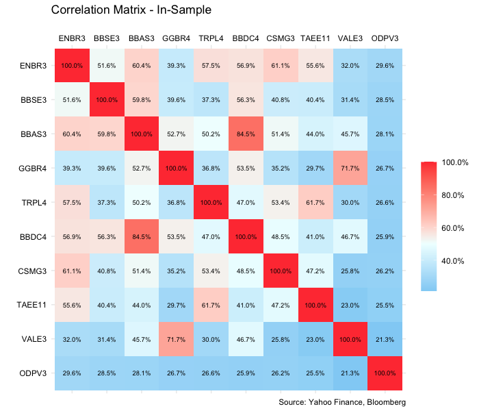
# In-Sample VAR-COV
insample_var_cov = cov(
  insample_returns %>% select(-date)
)

# In-Sample COR graphic
cor(insample_returns %>% select(-date)) %>%
  data.frame() %>%
  rownames_to_column("stock_r") %>%
  tibble() %>%
  gather(stock_c, value, -stock_r) %>%
  arrange(value) %>%
  mutate(
    stock_c = factor(stock_c, levels = unique(.$stock_c)),
    stock_r = factor(stock_r, levels = unique(.$stock_c) %>% rev())
  ) %>%
  ggplot(aes(stock_r, stock_c)) +
  geom_tile(aes(fill = value)) +
  scale_fill_gradient2(
    name = "",
    high = "brown1",
    mid = "azure",
    low = "deepskyblue2",
    midpoint = .5,
    labels = scales::percent_format(accuracy = .1)
  ) +
  labs(
    title = "Correlation Matrix - Training",
    x = "",
    y = "",
    caption = "Source: Yahoo Finance, Bloomberg"
  ) +
  theme_minimal() +
  theme(
    legend.position = "right",
    legend.key.height = unit(1, "cm"),
    legend.direction = "vertical",
    axis.text.x = element_text(colour = "black"),
    axis.text.y = element_text(colour = "black")
  ) +
  scale_x_discrete(position = "top") +
  geom_text(
    aes(label = scales::percent(value, accuracy = .1)),
    size = 2.5
  )
all_weights_db = c()
create_weights = function (wp){

  wp = as.integer(wp)

  new_weights_db = expand.grid(
    w1 = wp, w2 = wp, w3 = wp, w4 = wp,
    w5 = wp, w6 = wp, w7 = wp, w8 = wp,
    w9 = wp, w10 = wp) %>%
    mutate(
      total_weight = w1 + w2 + w3 + w4 + w5 + w6 + w7 + w8 + w9 + w10
    ) %>%
    mutate_if(is.numeric, ~ . / total_weight) %>%
    select(-total_weight)

  all_weights_db <<- all_weights_db %>%
    rbind(new_weights_db)
}

# Crate different possibilities of weights
# In the following case, the weights vary between 5% and 15% originally
# Weights are later adjusted by the sum of weights on order to always have the
# sum equals to 1 (Therefore, weights very between 3.5% and 25%)
create_weights(seq(50, 150, length.out = 5))

weights_info = all_weights_db %>%
  rename(weight = w1) %>%
  summarise(
    min_weight = min(weight),
    max_weight = max(weight)
  )

print(paste0(
  "Min weight per Stock: ",
  scales::percent(weights_info$min_weight, accuracy = .01),
  "; Max weight per Stock: ",
  scales::percent(weights_info$max_weight, accuracy = .01)
))
# Calculation of variance based on weights used
calculate_port_training_var = function (
  w1, w2, w3, w4, w5, w6, w7, w8, w9, w10
){

  weights = c(w1, w2, w3, w4, w5, w6, w7, w8, w9, w10)
  variance = weights %*% training_var_cov %*% weights
  return(variance)

}

# Vectorization of function in order to make it faster
calculate_port_training_var = Vectorize(calculate_port_training_var)

variances_db = all_weights_db %>%
  mutate(
    variance = calculate_port_training_var(
      w1, w2, w3, w4, w5, w6, w7, w8, w9, w10
    )
  )

penalized_variance_db = variances_db %>%
  mutate(
    penalizer = (
      w1 ^ 2 + w2 ^ 2 + w3 ^ 2 + w4 ^ 2 + w5 ^ 2
      + w6 ^ 2 + w7 ^ 2 + w8 ^ 2 + w9 ^ 2 + w10 ^ 2
    )
  ) %>%
  na.omit()
# Use lambda penalizer in order to understand which penalizer leads to the
# portfolio with the best predictions
best_penalized_port_calculation = function (selected_lambda){
i <<- i + 1
portfolios_db = penalized_variance_db %>%
mutate(penalized_variance = variance + penalizer * selected_lambda)
chosen_penalizer = min(portfolios_db$penalized_variance)
chosen_portfolio_weights = portfolios_db %>%
filter(penalized_variance == chosen_penalizer) %>%
arrange(variance) %>%
select(starts_with("w")) %>%
head(1)
chosen_port_weights_matrix = chosen_portfolio_weights %>%
as.matrix()
all_best_portfolios <<- all_best_portfolios %>%
rbind(
chosen_portfolio_weights %>%
mutate(lambda = scales::number(selected_lambda, accuracy = 0.000001))
)
testing_returns_matrix = testing_returns %>%
select(-date) %>%
as.matrix()
testing_portfolio_returns = (
testing_returns_matrix
%*% t(chosen_port_weights_matrix)
)%>%
data.frame() %>%
tibble() %>%
purrr::set_names(
paste0("l", scales::number(selected_lambda, accuracy = 0.000001))
) %>%
mutate(date = testing_returns$date) %>%
select(date, everything())
all_testing_portfolio_returns <<- all_testing_portfolio_returns %>%
full_join(testing_portfolio_returns, by = 'date')
setTxtProgressBar(
txtProgressBar(
min = 0, max = length(lambdas_list), style = 3
),
i
)
}
i = 0
all_best_portfolios = c()
all_testing_portfolio_returns = tibble(date = ymd())
# Try many different lambdas
lambdas_list = seq(0, 0.5, 0.0005)
# Multiplication of the lambda by the penalization factor
purrr::map(lambdas_list, ~ best_penalized_port_calculation(.))
lambdas = paste0(
"l", (
all_best_portfolios %>%
distinct(
w1, w2, w3, w4, w5, w6, w7, w8, w9,
w10, .keep_all = TRUE
)
)$lambda
)
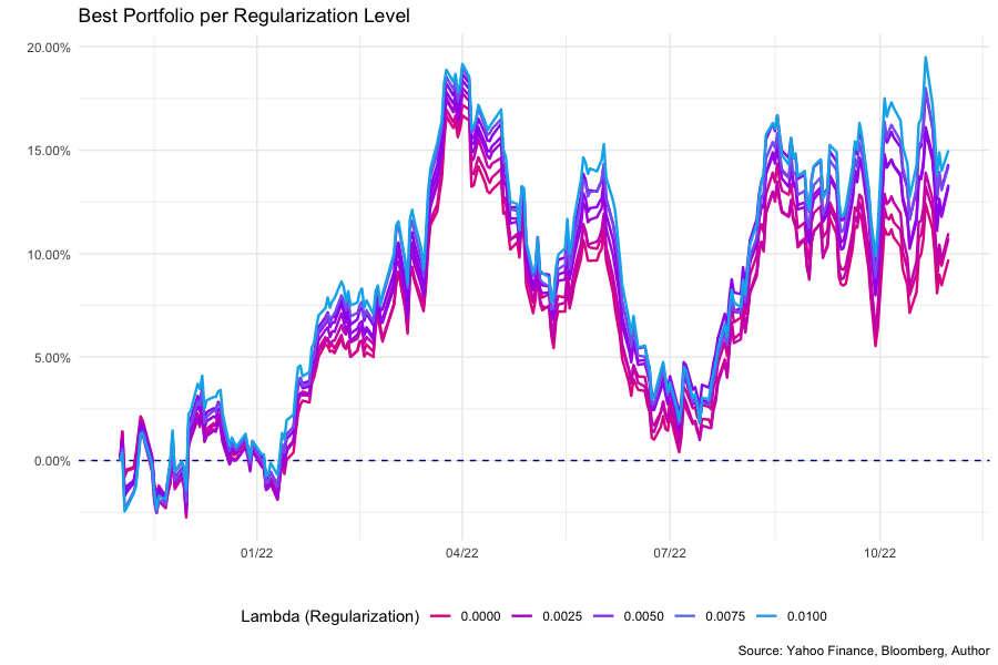
# Graphic showing portfolio acumulated returns by regularization (lambda) size
all_testing_portfolio_returns %>%
select(date, all_of(lambdas)) %>%
mutate_if(is.numeric, ~ cumprod(1 + .) - 1) %>%
add_row(date = min(.$date) - 1) %>%
mutate_if(is.numeric, ~ case_when(date == min(date) ~ 0, TRUE ~ .)) %>%
purrr::set_names(colnames(.) %>% str_remove("l")) %>%
gather(id, value, -date) %>%
mutate(id_color = as.numeric(id)) %>%
ggplot(aes(date, value)) +
geom_hline(
aes(yintercept = 0), linetype = 'dashed', color = "darkblue"
) +
geom_line(aes(color = id_color, group = id), size = 0.85) +
scale_y_continuous(labels = scales::percent_format(accuracy = 0.01)) +
scale_x_date(labels = scales::date_format("%m/%y")) +
labs(
title = "Best Portfolio per Regularization Level",
x = '',
y = '',
caption = 'Source: Yahoo Finance, Bloomberg, Author'
) +
scale_color_gradient2(
name = "Lambda (Regularization)",
high = "deepskyblue2",
mid = "purple",
midpoint = mean(
str_extract(lambdas, "[0-9]+(.)?([0-9]+)?") %>% as.numeric()
),
low = "brown1"
) +
guides(colour = guide_legend(nrow = 1)) +
theme_minimal() +
theme(
legend.position = 'bottom'
)
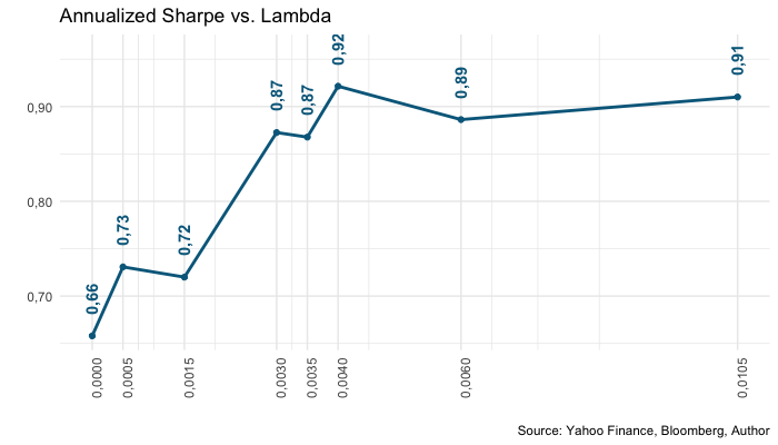
# Choice of best lambda by best Sharpe Ratio
penalizer_comparison = all_testing_portfolio_returns %>%
select(date, all_of(lambdas)) %>%
gather(lambda, value, -date) %>%
group_by(lambda) %>%
arrange(lambda, date) %>%
mutate(
cum_ret = cumprod(1 + value) - 1,
cum_ret = case_when(date == max(date) ~ cum_ret)
) %>%
fill(cum_ret, .direction = 'updown') %>%
group_by(lambda, cum_ret) %>%
summarise(volatility = sd(value) * sqrt(252)) %>%
mutate(lambda = str_remove(lambda, "l") %>% as.numeric()) %>%
mutate(
sharpe = (
((1 + cum_ret) ^ (252 / nrow(all_testing_portfolio_returns)) - 1)
/ volatility
)
) %>%
arrange(desc(sharpe))
best_lambda = penalizer_comparison$lambda[1]
print(paste("Selected Lambda:", scales::number(
best_lambda, accuracy = 0.00001, big.mark = '.', decimal.mark = ','
)))
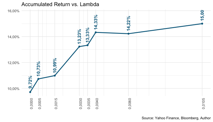
plot_statistic = function (column){
chosen_statistics = penalizer_comparison %>%
select(lambda, column + 1) %>%
purrr::set_names("lambda", "value")
chosen_statistics_plot = chosen_statistics %>%
ggplot(aes(x = lambda)) +
geom_line(aes(y = value), size = 1, color = "darkblue") +
geom_point(aes(y = value), color = "darkblue") +
scale_x_continuous(labels = scales::number_format(
accuracy = 0.0001, big.mark = '.', decimal.mark = ','
),
breaks = penalizer_comparison$lambda) +
labs(
x = '', y = '',
caption = 'Source: Yahoo Finance, Bloomberg, Author'
) +
theme_minimal()
if (column %in% c(1, 2)){
chosen_statistics_plot = chosen_statistics_plot +
labs(title = "Accumulated Return vs. Lambda") +
geom_text(
angle = 90,
aes(
y = value + (max(value) - min(value)) * 0.15,
label = scales::percent(
value, accuracy = 0.01, big.mark = '.', decimal.mark = ','
)
),
color = "darkblue", fontface = 2
) +
scale_y_continuous(labels = scales::percent_format(
accuracy = 0.01, big.mark = '.', decimal.mark = ','
))
} else {
chosen_statistics_plot = chosen_statistics_plot +
labs(title = "Annualized Sharpe vs. Lambda") +
scale_y_continuous(labels = scales::number_format(
accuracy = 0.01, big.mark = '.', decimal.mark = ',')) +
geom_text(
angle = 90,
aes(
y = value + (max(value) - min(value)) * 0.15,
label = scales::number(
value, accuracy = 0.01, big.mark = '.', decimal.mark = ','
)
),
color = "darkblue",
fontface = 2
)
}
if (column == 2){
chosen_statistics_plot = chosen_statistics_plot +
labs(title = "Volatilidade Anualizada vs. Lambda")
}
return(chosen_statistics_plot)
}
purrr::map(seq(1, 3), ~ plot_statistic(.))

# Lambda hyper parameter is found and now used for the in-sample in order to
# get best allocation for further allocation
calculate_port_insample_var = function (w1, w2, w3, w4, w5, w6, w7, w8, w9, w10){

  weights = c(w1, w2, w3, w4, w5, w6, w7, w8, w9, w10)
  variance = weights %*% insample_var_cov %*% weights
  return(variance)

}

# After finding the best penalizer (lambda), the calculation is done for
# the in-sample (training + testing)
calculate_port_insample_var = Vectorize(calculate_port_insample_var)

variances_insample_db = all_weights_db %>%
  mutate(variance = calculate_port_insample_var(
    w1, w2, w3, w4, w5, w6, w7, w8, w9, w10
  )) %>%
  mutate(
    penalizer = (
      w1 ^ 2 + w2 ^ 2 + w3 ^ 2 + w4 ^ 2 + w5 ^ 2 +
        w6 ^ 2 + w7 ^ 2 + w8 ^ 2 + w9 ^ 2 + w10 ^ 2
    ) * best_lambda,
    variance_penalized = variance + penalizer
  ) %>%
  arrange(variance_penalized, variance) %>%
  purrr::set_names(
    str_remove(stock_tickers, "[.]SA"), "Variance",
    "Penalizer", "Variance Penalized"
  )
variances_insample_db %>%
  head(1) %>%
  select(-"Variance", -contains("Penalize")) %>%
  gather("Ação", "Peso") %>%
  writexl::write_xlsx("portfolio_weights.xlsx")

# Results of in-sample
variances_insample_db %>%
  select(-contains("Variance"), -contains('Penalizer')) %>%
  head(1)

if (exists('variances_insample_db')){

  alocation_db = variances_insample_db %>%
    select(-contains("Variance"), -contains('Penalizer')) %>%
    head(1) %>%
    gather(id, value)

} else {

  alocation_db = read_excel("portfolio_weights.xlsx") %>%
    purrr::set_names("id", "value")

}

if (us_stock_opt == TRUE){

  alocation_db = alocation_db %>%
    left_join(
      us_stock_bdrs %>%
        rename(id = us_ticker), by = 'id'
    ) %>%
    select(-id) %>%
    rename(id = bdr)

}

# Graphic of in-sample allocation
alocation_db %>%
  mutate(id = id %>% str_remove("[.]SA")) %>%
  arrange(id) %>%
  mutate(acum_value = 1 - cumsum(value)) %>%
  ggplot(aes(x=2, y=value, fill=id)) +
  geom_col() +
  coord_polar("y", start = 0) +
  theme_minimal() +
  theme(
    panel.background = element_blank(),
    axis.line = element_blank(),
    axis.text = element_blank(),
    axis.ticks = element_blank(),
    axis.title = element_blank(),
    plot.title = element_text(hjust = 0.5, vjust = -1.5),
    panel.grid.major = element_blank(),
    panel.grid.minor = element_blank()
  ) +
  scale_y_continuous(limits = c(0, 1.0)) +
  geom_label(
    aes(
      y = acum_value, x = 2.2,
      label = scales::percent(value, accuracy = 0.01),
      fill = id
    ),
    color = 'white', fontface = 2,
    position = position_dodge2(width = .1),
    size = 2,
    show.legend = FALSE
  ) +
  labs(
    title = 'In-Sample Best Allocation',
    x = '',
    y = '',
    caption = 'Source: Yahoo Finance, Bloomberg, Author'
  ) +
  scale_fill_manual(
    name = "",
    values = c(
      "chocolate1",
      "cornflowerblue",
      "coral",
      "springgreen3",
      "brown1",
      "aquamarine3",
      "deeppink1",
      "cyan3",
      "darkorchid2",
      "cadetblue2"
    )
  ) +
  xlim(0.5, 2.5) +
  guides(fill = guide_legend(ncol = 1))
