getting started
[[TOC]]
Here we provide an introduction on how to set up and conduct inverse modelling runs with PROPTI. This tutorial is based on the simulation software Fire Dynamics Simulator FDS, the optimisation algorithm is the Shuffled Complex Evolutionary algorithm SCEUA from the SPOTPY Python framework.
Note: This example is built around an input file that is provided with FDS (tga_analysis.fds). The experimental data used here as target is fabricated and the result of a simulation of the original FDS example file.
Detailed technical information on the PROPTI classes, functions and parameters can be found in the Technical Documentation.
For a very basic run of the inverse modelling process IMP, utilising PROPTI, one needs to set up three different files. One file needs to contain the data that is used for the optimisation algorithm as a target. This target data is most likely to be data from an experiment, that is ought to be recreated by simulation. Furthermore, there needs to be a template of the input file for the simulation software. This template contains markers, specific character chains, embedded in the regular text of the file. PROPTI will parse the template in a later step and exchange the markers with values provided by the optimisation algorithm. Finally, an input file for PROPTI is needed. It contains instructions on what specific parameters the IMP shall follow, what simulation software and optimisation algorithm to use, what files contain target data and which template to be used.
In general, PROPTI itself works in multiple steps, with these three steps being the foundation: "prepare", "run" and "analysis". After the files described above have been created, PROPTI needs to perform a preparation step. There, it reads the information contained in the PROPTI input file. It creates a binary file, called propti.pickle.init, that contains all the provided information for this project. Afterwards, it collects the simulation template and target data files, creates a working directory with sub-directories and copies the necessary files there. In the sub-directories the actual calculations will be performed and they will deleted automatically after each calculation has finished. PROPTI only stores parts of the simulation results, that are necessary for the respective project.
When the preparation has finished, the IMP run can be started. PROPTI will then look up the needed information stored in the propti.pickle.init, create simulation input files, based on parameters provided by the optimisation algorithm, and write them to calculation directories. It will start the simulations, retrieve the results and feed them back to the algorithm. Afterwards it will clean up and delete the files of the finished simulation. The cycle will begin again and repeats itself. The process is stopped when the algorithm signals that it has met its termination criteria.
During the IMP a data base is created in form of a comma separated value CSV file. It contains all guess vectors that have been simulated, as well as their respective simulation responses. For now, the creation of the data base is handled by SPOTPY, because PROPTI does not provide its own means for data base creation, yet.
After the IMP is completed, or even during the run, the progress can be assessed. PROPTI provides a collection of functions that can extract certain information in a relatively simple fashion. In principal, they are reading the content of the propti.pickle.init, as well as the propti_db.csv, and use this information to create basic plots or create simulation input files with the best parameter set, for instance. The user is encouraged to investigate the inner workings of said functions and use them to build their own functions, if the desired operation is not on hand.
Effort was also put into providing some means of sensitivity analysis of the optimisation parameters. By performing the analysis the user may be able to reduce the amount of parameters needed for the IMP, with the benefit of saving computational resources. Even the reduction by one or two parameters may lead to significant savings.
The three necessary files (FDS template, fabricated experimental data and PROPTI input) for this tutorial are provided in the propti/examples/tga_analysis_01/ directory.
For this tutorial, mock-up experimental data is provided. They are the result of a simulation of the example file tga_analysis.fds that is provided with FDS. The file containing the fabricated experimental data is called tga_experimental_data.csv. It is a comma separated value CSV file that contains six columns. Labels for the individual columns are provided in the first line and will be used to identify specific columns later on.
For this example, FDS is utilised as simulation software. The simulation input file template is called template_tga_01.fds and can be found in propti/examples/tga_analysis_01/. An input file template for FDS, or any other simulation software, is created as follows: At first, an input file needs to be created that defines the desired simulation setup completely. It should contain all necessary aspects, like geometries, devices material model and so forth. When this file has been created it should be tested, to figure out if is processed correctly by FDS (or what ever program one intents to use) and does not rise any errors. After the testing concluded successful, values in the FDS input file can be substituted by placeholders. These function as markers for PROPTI, such that it can identify specific locations where values need to be written into the template.
As per convention, placeholders are simply character chains (strings) that are to be encapsulated by '#' characters. Between the two '#' an arbitrary string can be written, for example '#SoylentGreen#'.
For this example we try to generate material parameters that produce a simulation response which is similar to a (fictional) experiment that was conducted. The FDS input file describes a simulation setup of a thermo-gravimetric analysis. Four material components are used to describe the material. Component 1 is the main material which contains some water. When heated, the water will evaporate, also component 1 will produce combustible gas and another material, simply called component 2. In turn, component 2 will produce combustible gas and a residue.
Let's assume, we have identified that component 1 and 2 are important for our problem, specifically the reference rate and the reference temperature for each are the most influential parameters. That leaves us with four unknown parameters that need to be varied. In the prepared FDS input file, we write placeholders at the locations for the four respective parameters, we use the abbreviation "rt" for the reference temperature and "rr" for the reference rate, followed by a "c01" or "c02" depending on the component. These for markers are then encapsulated "#", for example: "#rtc01#".
Below is an example of how it looks in the FDS input file template.
&MATL ID                    = 'component 1'
      EMISSIVITY            = 1.0
      DENSITY 	            = 500.
      CONDUCTIVITY          = 0.20
      SPECIFIC_HEAT         = 1.0
      N_REACTIONS           = 1
      REFERENCE_TEMPERATURE = #rtc01#
      REFERENCE_RATE        = #rrc01#
      HEATING_RATE          = #hr#
      NU_SPEC 	            = 0.60
      SPEC_ID               = 'CELLULOSE'
      NU_MATL               = 0.40
      MATL_ID               = 'component 2'
      HEAT_OF_REACTION      = 1000. /
We also added a placeholder for the heating rate, seen above, and for the character ID (CHID), seen below. These two placeholders demonstrate the possibility to provide parameters that are not directly part of the optimisation process. These are more like model or environment parameters (maybe meta-parameters), and could also be used if the same material was tested with different heating rates (see example 2).
&HEAD CHID='#CHID#', TITLE='TGA tutorial' /
The finalised FDS input template is shown below.
&MESH IJK=3,1,4, XB=-2,2,-0.5,0.5,0,1 /

&TIME T_END=60. /

&REAC FUEL='CELLULOSE', C=6, H=10, O=5, SOOT_YIELD=0.015 /
&SPEC ID='WATER VAPOR' /

&VENT XB=-1,1,-0.5,0.5,0.0,0.0, SURF_ID='SAMPLE' /

&SURF ID             = 'SAMPLE'
      TGA_ANALYSIS   = .TRUE.
      COLOR          = 'RED'
      THICKNESS      = 0.01
      MATL_ID(1,1) = 'component 1'
      MATL_ID(1,2) = 'water'
      MATL_MASS_FRACTION(1,1) = 0.90
      MATL_MASS_FRACTION(1,2) = 0.10 /

&MATL ID                    = 'component 1'
      EMISSIVITY            = 1.0
      DENSITY 	            = 500.
      CONDUCTIVITY          = 0.20
      SPECIFIC_HEAT         = 1.0
      N_REACTIONS           = 1
      REFERENCE_TEMPERATURE = #rtc01#
      REFERENCE_RATE        = #rrc01#
      HEATING_RATE          = #hr#
      NU_SPEC 	            = 0.60
      SPEC_ID               = 'CELLULOSE'
      NU_MATL               = 0.40
      MATL_ID               = 'component 2'
      HEAT_OF_REACTION      = 1000. /

&MATL ID                    = 'component 2'
      EMISSIVITY            = 1.0
      DENSITY 	            = 500.
      CONDUCTIVITY          = 0.20
      SPECIFIC_HEAT         = 1.0
      N_REACTIONS           = 1
      REFERENCE_TEMPERATURE = #rtc02#
      REFERENCE_RATE        = #rrc02#
      HEATING_RATE          = #hr#
      NU_SPEC 	            = 0.85
      SPEC_ID               = 'CELLULOSE'
      NU_MATL               = 0.15
      MATL_ID               = 'residue'
      HEAT_OF_REACTION      = 1000. /

&MATL ID = 'water'
      DENSITY = 1000.
      CONDUCTIVITY = 0.1
      SPECIFIC_HEAT= 4.184
      N_REACTIONS = 1
      REFERENCE_TEMPERATURE = 100.
      REFERENCE_RATE = 0.0016
      HEATING_RATE = #hr#
      NU_SPEC = 1.0
      SPEC_ID = 'WATER VAPOR'
      HEAT_OF_REACTION= 2500. /

&MATL ID                    = 'residue'
      DENSITY               = 200.
      CONDUCTIVITY          = 0.20
      SPECIFIC_HEAT         = 1.0 /

&TAIL /
Now, since the simulation software input file and the experimental data file are prepared, it is time to set up the IMP. The example file is called input.py and can be found in propti/examples/tga_analysis_01/.
Within the PROPTI input file there are in general three types of parameter sets need to be specified:
- Optimisation parameter set
- Simulation setup set
- Properties for the optimiser
The optimisation parameters are the ones that the optimisation algorithm has direct access to, and that are adjusted by the algorithm. A simulation setup is a set of information that describes a simulation completely. That means generally the simulation input template, the optimisation parameters and meta parameters. The optimiser properties deliver information to the optimiser of what algorithm to use or how many repetitions to perform, for example.
At first we provide some general information that will be needed throughout this input file. These are items like template file names or target data files. Also, some general meta information like the file names could be given here.
# Input file template for the simulation software.
template_file = "template_tga_01.fds"

# File containing the experimental data that is used as target during the
# inverse modelling process.
exp_data_file = "tga_experimental_data.csv"

# Character ID used to identify the files connected to one simulation.
CHID = 'TGA_analysis_01'

#
TEND = 9360
We need to specify the optimisation parameters. For each parameter we have to specify a name, a place-holder, and the limits of the sample range. The parameter names are used for internal referencing. The place-holder will be used to replace the markers which have been specified in the FDS template. The "#" character will be added by PROPTI automatically, thus can be omitted here. For the optimisation process lower and upper boundaries are needed to provide the algorithm a range to sample parameters values from - the min and max values.
# define the optimisation parameter
op1 = pr.Parameter(name='ref_temp_comp_01',
                   place_holder='rtc01',
                   min_value=200, max_value=400)
op2 = pr.Parameter(name='ref_rate_comp_01',
                   place_holder='rrc01',
                   min_value=0.001, max_value=0.01)
op3 = pr.Parameter(name='ref_temp_comp_02',
                   place_holder='rtc02',
                   min_value=300, max_value=600)
op4 = pr.Parameter(name='ref_rate_comp_02',
                   place_holder='rrc02',
                   min_value=0.001, max_value=0.01)

# Collect all the defined parameters from above, just for convenience.
set_of_parameters = [op1, op2, op3, op4]
After their definition, the parameters are collected within a parameter set to be provided to propti_prepare.py in the next step.
# Definition of parameters, which is used by `propti_prepare.py` later on.
# It has no further meaning here.
ops = pr.ParameterSet(name="Optimisation parameters",
                      params=set_of_parameters)
Now, the model parameters need to be defined which describe the experimental setup. They consist of the meta data and the parameters to be optimised. Since we collected the optimisation parameters into a list before, we just need to add this list to the set. All other data has to be added similar as described above.
# Definition of general model parameters, including optimisation parameters.
mps0 = pr.ParameterSet(name="Environment and\n"
                            "Optimisation parameters",
                       params=set_of_parameters)
mps0.append(pr.Parameter(name='heating rate', place_holder='hr', value=10))
mps0.append(pr.Parameter(name='chid', place_holder='CHID', value=CHID))
Afterwards, the relationship between the simulation output data and the experimental data needs to be specified, as shown below. For both, the model data and the experimental data, the names of the files have to be specified. The files have to be formatted as csv files, with a header line containing the label of each data column. This allows the specific columns to be accessed via their respective label. We make also use of the character Id defined in the beginning, to read the simulation result files dynamically.
# Define model-experiment data relation
r = pr.Relation()
r.model.file_name = "{}_tga.csv".format(CHID)
r.model.label_x = 'Time'
r.model.label_y = 'MLR'
r.model.header_line = 1
r.experiment.file_name = exp_data_file
r.experiment.label_x = 'Time'
r.experiment.label_y = 'MassLossRate'
r.experiment.header_line = 0
Now, the definition range is needed to describe which parts of the experimental and model data are to be used for the comparison. This is specifically interesting, when model and simulation data were taken with different time intervals between their respective data points.
# Define definition range for data comparison
r.x_def = np.arange(0., TEND, 12)
Based on the information defined above, the simulation setup will be created. A name is used for internal referencing. A working directory needs to be specified, which will be created automatically later on, and in which the computation takes place. Furthermore, the FDS template name and the model parameters (from above) are needed, as well as the relationship between the model and experimental data is expected. Finally, the program for conducting the simulations (here FDS).
# Create simulation setup object
s = pr.SimulationSetup(name='tga_analysis_01',
                       work_dir='tga_analysis_run_01',
                       model_template=template_file,
                       model_parameter=mps0,
                       model_executable='fds',
                       relations=r)
It is possible to create multiple simulation setups for a single IMP run. This comes in handy when the set of optimisation parameters is desired to be tested under different conditions at once, for example. Further information on this feature can be found in another example.
Even with only on simulation setup, it is necessary to store it into a simulation setup set.
# Define empty simulation setup set
setups = pr.SimulationSetupSet()
# Append above object to simulation setup set
setups.append(s)
Finally, there is some information that is to be provided to the optimiser. Here ,it would be sufficient to define an algorithm and the desired amount repetitions for a basic IMP run. As example the shuffled complex evolutionary algorithm, implemented in SPOTPY was chosen. The user has control over the amount of complexes for the SCEUA, with the parameter ngs, default value is shown here.
Note: The execution of the SCEUA happens in two different phases in SPOTPY. Phase one is the "burn-in", phase two is the "complex-evolution". During burn-in, random parameters are generated and one generation worth of guess vectors are generated. Data for each of these guess vectors are written to the database file immediately. However, during complex-evolution, SPOTPY buffers the results internally for each complex to process the information. Only AFTER the information of a complex is processed, it will be written to the database. Thus, for large complexes and (possibly) long duration simulations, the update frequency of the database can be quite low, possibly hours.
# Provide parameter values for the optimiser, some of the default values are
# highlighted here.
optimiser = pr.OptimiserProperties(algorithm='sceua',
                                   repetitions=1000,
                                   ngs=len(set_of_parameters),
                                   backup_every=100,
                                   db_name='propti_db',
                                   db_type='csv',
                                   db_precision=np.float64,
                                   mpi=False)
However, some more parameters are shown here, with their default values. The backup_every sets a number of repetitions after which the state of the IMP is written to a file. With this file the IMP can be restarted, for instance after a system crash or if the computing resources require time tokens, often found in supercomputing facilities, and long lasting IMP runs would exceed the token's time frame.
Note: The specific functionality of the backup is dependent on the utilised algorithm
Some options of the data base are exposed to the user as well. The name (db_name), the file type (db_type) and the float value precision (db_precision) can be customised. For now, only CSV is a possible format.
After the necessary files (simulation template, experimental data, PROPTI input) have been created, as discussed above, the first PROPTI step can be performed, which is implemented into the script propti_prepare.py. Information provided by input.py controls the preparation step. Assuming, the user starts in the example directory propti/examples/tga_analysis_01/, the preparation step is performed with the following command line input, providing the input.py as a parameter:
python3 ../../propti_prepare.py input.pyPROPTI will then create a binary file propti.pickle.init, which is used to store the initialised Python objects. Furthermore, it creates a sub directory, on the level where input.py is located, and copies the simulation template, as well as the experimental data files there. Also, a log file to monitor the PROPTI progress will be written.
The preparation is the basic step for the PROPTI process, all the other steps build on it. Further steps will send queries to propti.pickle.init retrieve needed information, like paths to working directories or which optimisation algorithm to use.
A sensitivity analysis will help us determine which parameters in the numerical model strongly affect our simulation. This allows us to reduce the number of model parameters during the subsequent optimisation process, thereby saving up on valuable computation time.
For the purpose of sensitivity analysis, we use the FAST algorithm (Fourier Amplitude Sensitivity Analysis) provided by SPOTPY. Once the process of preparation (propti_prepare.py) is executed, a sensitivity analysis can be performed for the parameters in the input file. In the working directory we run:
python3 ../../propti_sense.py .Upon execution of the script, the FAST algorithm generates the following (partial) output, with the first and total SOBOL sensitivity index values for the 4 parameters considered. The total SOBOL sensitivity index (ST) determines the total effect of a particular parameter taking in consideration, its dependency to the variance of the remaining parameters in the simulation. We thus consider this value as the total sensitivity of a model parameter to the simulation.
720 of 724 (best like=0.000577571) est. time remaining: 00:00:20
721 of 724 (best like=0.000577571) est. time remaining: 00:00:13
722 of 724 (best like=0.000577571) est. time remaining: 00:00:07
723 of 724 (best like=0.000577571) est. time remaining: 00:00:00
724 of 724 (best like=0.000577571) est. time remaining: 23:59:53
End of sampling
Best run at 122 of 724 (best like=0.000577571) with parameter set:
[3.97017048e+02 9.16963457e-03 3.73426125e+02 9.16963457e-03]
Duration:4801.22 s
724
Parameter First Total
rtc01 0.346703 0.577154
rrc01 0.342023 0.429666
rtc02 0.044371 0.219820
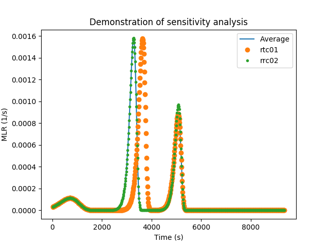
rrc02 0.027654 0.058417Based on the sensitivity values, the user is able to see that rrc02 has the lowest of all sensitivities. In the following, we have compared mass loss rate (MLR) curves of three simulations namely, an average curve, increasing only rtc01 by 10% from its average value and increasing only rrc02 by 10%. The results here are quite clear. Changes to rrc02 have a smaller effect on the overall curve compared to rtc01.
Once the decision to remove certain parameters has been made, the user must again edit the original input.py file, make the necessary changes before running the propti_prepare.py script. Either, the user adjusts the simulation template and removed the parameters from the input.py or the specific parameters are moved from the optimisation parameters to the meta parameters that describe the simulation environment.
Additional note:
Once the propti_prepare.py script has been executed, the respective propti.pickle.init file is read by propti_sense.py and the necessary changes are made to execute the FAST algorithm on the optimization parameters. Importantly, propti.pickle.init is not altered and remains in its original state. Upon execution of the script, the user may realise that even though certain parameters are less sensitive, they may be responsible for certain 'special' effects the user is trying to capture.
Therefore, it is in the users' province to make these considerations, and only then decide which parameters they want to keep during the subsequent optimisation process.
The execution of the IMP job is implemented into the propti_run.py script. To run the job, the following command has to be executed, assuming the example directory propti/examples/tga_analysis_01/ as starting point.
python3 ../../propti_run.py .In this directory, propti_run.py will look for the propti.pickle.init and read information on the IMP from it. Within the sub-directory, which had been created by the preparation step, a further sub-directory is created. This new calculation directory is used during the simulation, and files created by the simulation software are stored here. When the simulation has concluded successfully, the resulting data, defined in the Relation, will be extracted and the remaining files, including the directory, are removed. Part of the calculation directories name is randomly generated, which is important when parallel execution is desired (will be described in another example).
This section expands on information, already provided in the "PROPTI Input File" section.
SPOTPY allows the user to backup data generated during an optimisation process. This is especially beneficial, in an event of a system crash or when the utilised computing resources rely on time tokens. These token systems are often found in large scale computing facilities, like supercomputers. This is done by setting two variables, namely: breakpoint and backup_every_rep. A breakfile is then created, which includes data about the optimisation process.
Relevant Variables:
breakpoint (default = None): checks whether a breakfile is already present in the working directory and reads it. (possible values: read, write, readandwrite)
backup_every_rep (default = 100): is the number of repetitions of the optimisation process before a backup is made.
Note: If the optimisation process is finished, and the breakfile is present in the working directory, the optimisation process will recognize it and not continue further.
Importantly, within PROPTI the process of file checking is done automatically before calling the optimisation algorithm (via /propti/spotpy_wrapper.py) when propti_run.py is executed. The user is thus not required to input any variables.
PROPTI provides basic means of analysing and processing of the IMP results. For one, it is able to provide a variety of plots of different items. Furthermore, some basic data extraction allows to retrieve parameter sets from the data base file. The extracted data is then written into template files, specified by the user.
The whole concept of propti_analysis.py revolves around the fact, that all necessary information of an IMP run is stored in the propti.pickle.init. Thus, propti_analysis.py can query propti.pickle.init to automatically find the information needed to perform the plotting or extraction commands.
Note: For now the analysis script is very much designed for a usage in concert with the SCEUA implementation of SPOTPY. Expect changes in the future.
Designed as a script accessed from the command line, propti_analysis.py can be provided with options, in the common --option argument way. In general:
JohnDoe@morgue:~/some/working/directory$ SomeProgram --option argumentFor the usage of the propti_analysis.py options, the argument is the location of the propti.pickle.init. Assuming the user starts from the projects directory as the working directory, the arguments will simply be a period .. See below, for more specific examples.
The propti_analyse.py script creates a sub-directory within the directory of the project, which is named Analysis. There, it stores the output that it creates, in appropriate sub-directories.
The results of the plotting functions are stored within /Analysis/Plots.
A convenient function is accessed with the option --dump_plots and needs a further argument for the location of the propti.pickle.init. In our case this file is located in the working directory directly, thus the argument will be .. The function automatically creates a variety of different plots:
- scatter plot for each parameter value over the course of the IMP run
- scatter plot of the fitness value, to provide an overview over its development during the IMP
- scatter plots of the best parameter values per generation, for each parameter
- collection of box plots, one per generation
An example on how to call it is provided below (note the . at the end of the line):
JohnDoe@morgue:~/path/to/tga_analysis_01$ python3 ~/path/to/propti/propti_analyse.py --dump_plots .The results of the data extraction functions are stored within /Analysis/Extractor.
With --create_best_input, a simulation input file will be created, using the simulation input template, the best parameter set from the data base and the meta parameters from the propti.pickle.init. Within Extractor, a sub directory named CurrentBestParameter will be created. There, further sub-directories are created on demand, named after the repetition of the used parameter set. This is especially helpful, when this functionality is used to occasionally check the IMP, basically snapshots. In that case, the "best parameter set" may change over time, but the user might want to keep the files.
A more generic result can be achieved with --extract_data. It will lead to processing the database and extract the information of the best parameter set per generation. This creates a CSV file, containing the number of the complex, the fitness value, the best parameter set and the repetition number. The resulting CSV file is stored in Extractor, within a sub directory named BestParameterGeneration.
The above CSV file can be used to create simulation input files with --extractor_sim_input. Copies of the simulation input template will then be filled with best parameter sets per generation and named after the repetition. The resulting files are written to directories which are themselves named after the respective repetition. They are sub-directories in ExtractorSimInput.
Plot of fitness against evaluations

Plot of first optimisation parameter value against evaluations
Zenodo DOI: