Since 2018, pre-training has without a doubt become one of the hottest research topics in Natural Language Processing (NLP). By leveraging generalized language models like the BERT, GPT and XLNet, great breakthroughs have been achieved in natural language understanding. However, in sequence to sequence based language generation tasks, the popular pre-training methods have not achieved significant improvements. Now, researchers from Microsoft Research Asia have introduced MASS—a new pre-training method that achieves better results than BERT and GPT.


- https://deep-learning-drizzle.github.io/
- https://madewithml.com/
- http://biostat.mc.vanderbilt.edu/wiki/Main/RmS
- https://nlpprogress.com/
- Tracking Progress in Natural Language Processing
- A curated list of resources dedicated to Natural Language Processing (NLP)
- https://www.cs.cmu.edu/~rsalakhu/
- https://github.com/harvardnlp
- https://nlpoverview.com/
- Stat232A: Statistical Modeling and Learning in Vision and Cognition
- https://textprocessing.github.io/
- https://nlpforhackers.io/
- http://www.cs.yale.edu/homes/radev/dlnlp2017.pdf
- https://handong1587.github.io/deep_learning/2015/10/09/nlp.html
- https://cla2018.github.io/dl4nlp_roth.pdf
- https://deep-learning-nlp.readthedocs.io/en/latest/
- https://zhuanlan.zhihu.com/c_188941548
- https://allennlp.org/
- http://aan.how/
- http://www.cs.yale.edu/homes/radev/
- http://www.cs.cmu.edu/~bishan/pubs.html
- http://web.stanford.edu/class/cs224n/index.html
- https://explosion.ai/
The general building blocks of their model, however, are still found in all current neural language and word embedding models. These are:
- Embedding Layer: a layer that generates word embeddings by multiplying an index vector with a word embedding matrix;
- Intermediate Layer(s): one or more layers that produce an intermediate representation of the input, e.g. a fully-connected layer that applies a non-linearity to the concatenation of word embeddings of
$n$ previous words; - Softmax Layer: the final layer that produces a probability distribution over words in
$V$ .
The softmax layer is a core part of many current neural network architectures. When the number of output classes is very large, such as in the case of language modelling, computing the softmax becomes very expensive.
Word are always in the string data structure in computer.
Language is made of discrete structures, yet neural networks operate on continuous data: vectors in high-dimensional space. A successful language-processing network must translate this symbolic information into some kind of geometric representation—but in what form? Word embeddings provide two well-known examples: distance encodes semantic similarity, while certain directions correspond to polarities (e.g. male vs. female). There is no arithmetic operation on this data structure. We need an embedding that maps the strings into vectors.
Language Modeling (LM) estimates the probability of a word given the previous words in a sentence:
- Probability and Structure in Natural Language Processing
- Probabilistic Models in the Study of Language
- CS598 jhm Advanced NLP (Bayesian Methods)
- Statistical Language Processing and Learning Lab.
- Bayesian Analysis in Natural Language Processing, Second Edition
- Probabilistic Context Grammars
- https://ofir.io/Neural-Language-Modeling-From-Scratch/
- https://staff.fnwi.uva.nl/k.simaan/D-Papers/RANLP_Simaan.pdf
- https://staff.fnwi.uva.nl/k.simaan/ESSLLI03.html
- http://www.speech.cs.cmu.edu/SLM/toolkit_documentation.html
- http://www.phontron.com/kylm/
- http://www.lemurproject.org/lemur/background.php
- https://meta-toolkit.org/
- https://github.com/renepickhardt/generalized-language-modeling-toolkit
- http://www.cs.cmu.edu/~nasmith/LSP/
The Neural Probabilistic Language Model can be summarized as follows:
- associate with each word in the vocabulary a distributed word feature vector (a real valued vector in
$\mathbb{R}^m$ ), - express the joint probability function of word sequences in terms of the feature vectors of these words in the sequence, and
- learn simultaneously the word feature vectors and the parameters of that probability function.
When a word
- https://www.cs.bgu.ac.il/~elhadad/nlp18/nlp02.html
- http://josecamachocollados.com/book_embNLP_draft.pdf
- https://arxiv.org/abs/1906.02715
- Project Examples for Deep Structured Learning (Fall 2018)
- https://ruder.io/word-embeddings-1/index.html
- https://carl-allen.github.io/nlp/2019/07/01/explaining-analogies-explained.html
- https://arxiv.org/abs/1901.09813
- Analogies Explained Towards Understanding Word Embeddings
- https://pair-code.github.io/interpretability/bert-tree/
- https://pair-code.github.io/interpretability/context-atlas/blogpost/
- http://disi.unitn.it/moschitti/Kernel_Group.htm
- https://lilianweng.github.io/lil-log/2018/06/24/attention-attention.html
- Attention Is All You Need
- https://arxiv.org/pdf/1811.05544.pdf
- https://arxiv.org/abs/1902.10186
- https://arxiv.org/abs/1906.03731
- https://arxiv.org/abs/1908.04626v1
- 遍地开花的 Attention,你真的懂吗? - 阿里技术的文章 - 知乎
- https://www.jpmorgan.com/jpmpdf/1320748255490.pdf
- Understanding Graph Neural Networks from Graph Signal Denoising PerspectivesCODE
- Attention and Augmented Recurrent Neural Networks
- https://www.dl.reviews/
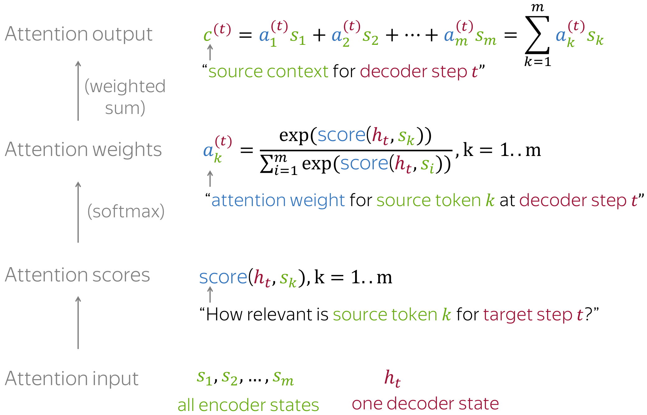
Attention distribution is a probability distribution to describe how much we pay attention into the elements in a sequence for some specific task.
For example, we have a query vector
- https://chulheey.mit.edu/
- https://arxiv.org/abs/2101.11347
- https://linear-transformers.com/
- https://github.com/idiap/fast-transformers
The attention function between different input vectors is calculated as follows:
- Step 1: Compute scores between different input vectors and query vector
$S_N$ ; - Step 2: Translate the scores into probabilities such as
$P = \operatorname{softmax}(S_N)$ ; - Step 3: Obtain the output as aggregation such as the weighted value matrix with
$Z = \mathbb{E}_{z\sim p(\mid \mathbf{X}, \mathbf{q} )}\mathbf{[x]}$ .
There are diverse scoring functions and probability translation function, which will calculate the attention distribution in different ways.
Efficient Attention, Linear Attention apply more efficient methods to generate attention weights.
Key-value Attention Mechanism and Self-Attention use different input sequence as following
$$\operatorname{att}(\mathbf{K, V}, \mathbf{q}) =\sum_{j=1}^N\frac{s(\mathbf{K}_j, q)\mathbf{V}j}{\sum{i=1}^N s(\mathbf{K}_i, q)}$$
where
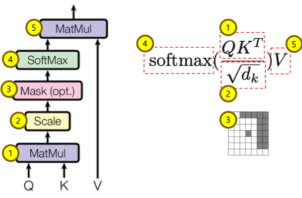
Each input token in self-attention receives three representations corresponding to the roles it can play:
- query - asking for information;
- key - saying that it has some information;
- value - giving the information.
We compute the dot products of the query with all keys, divide each by square root of key dimension
Soft Attention: the alignment weights are learned and placed “softly” over all patches in the source image; essentially the same type of attention as in Bahdanau et al., 2015. And each output is derived from an attention averaged input.
- Pro: the model is smooth and differentiable.
- Con: expensive when the source input is large.
Hard Attention: only selects one patch of the image to attend to at a time, which attends to exactly one input state for an output.
- Pro: less calculation at the inference time.
- Con: the model is non-differentiable and requires more complicated techniques such as variance reduction or reinforcement learning to train. (Luong, et al., 2015)
Soft Attention Mechanism is to output the weighted sum of vector with differentiable scoring function:
where
In practice, we compute the attention function on a set of queries simultaneously, packed together into a matrix
- https://ayplam.github.io/dtca/
- Fast Pedestrian Detection With Attention-Enhanced Multi-Scale RPN and Soft-Cascaded Decision Trees
- DTCA: Decision Tree-based Co-Attention Networks for Explainable Claim Verification
Hard Attention Mechanism is to select most likely vector as the output
$$\operatorname{att}(\mathbf{X}, \mathbf{q}) = \mathbf{x}j$$
where $j=\arg\max{i}\alpha_i$.
It is trained using sampling method or reinforcement learning.
- Effective Approaches to Attention-based Neural Machine Translation
- https://github.com/roeeaharoni/morphological-reinflection
- Surprisingly Easy Hard-Attention for Sequence to Sequence Learning
The softmax mapping is elementwise proportional to
Sparse Attention Mechanism is aimed at generating sparse attention distribution as a trade-off between soft attention and hard attention.
- Generating Long Sequences with Sparse Transformers
- Sparse and Constrained Attention for Neural Machine Translation
- https://github.com/vene/sparse-structured-attention
- https://github.com/lucidrains/sinkhorn-transforme
- http://proceedings.mlr.press/v48/martins16.pdf
- https://openai.com/blog/sparse-transformer/
- Sparse and Continuous Attention Mechanisms
GAT introduces the attention mechanism as a substitute for the statically normalized convolution operation.

- Graph Attention Networks
- https://petar-v.com/GAT/
- https://docs.dgl.ai/en/0.4.x/tutorials/models/1_gnn/9_gat.html
- https://dsgiitr.com/blogs/gat/
- https://www.ijcai.org/Proceedings/2019/0547.pdf
Representation learning forms the foundation of today’s natural language processing system; Transformer models have been extremely effective at producing word- and sentence-level contextualized representations, achieving state-of-the-art results in many NLP tasks. However, applying these models to produce contextualized representations of the entire documents faces challenges. These challenges include lack of inter-document relatedness information, decreased performance in low-resource settings, and computational inefficiency when scaling to long documents. In this talk, I will describe 3 recent works on developing Transformer-based models that target document-level natural language tasks.
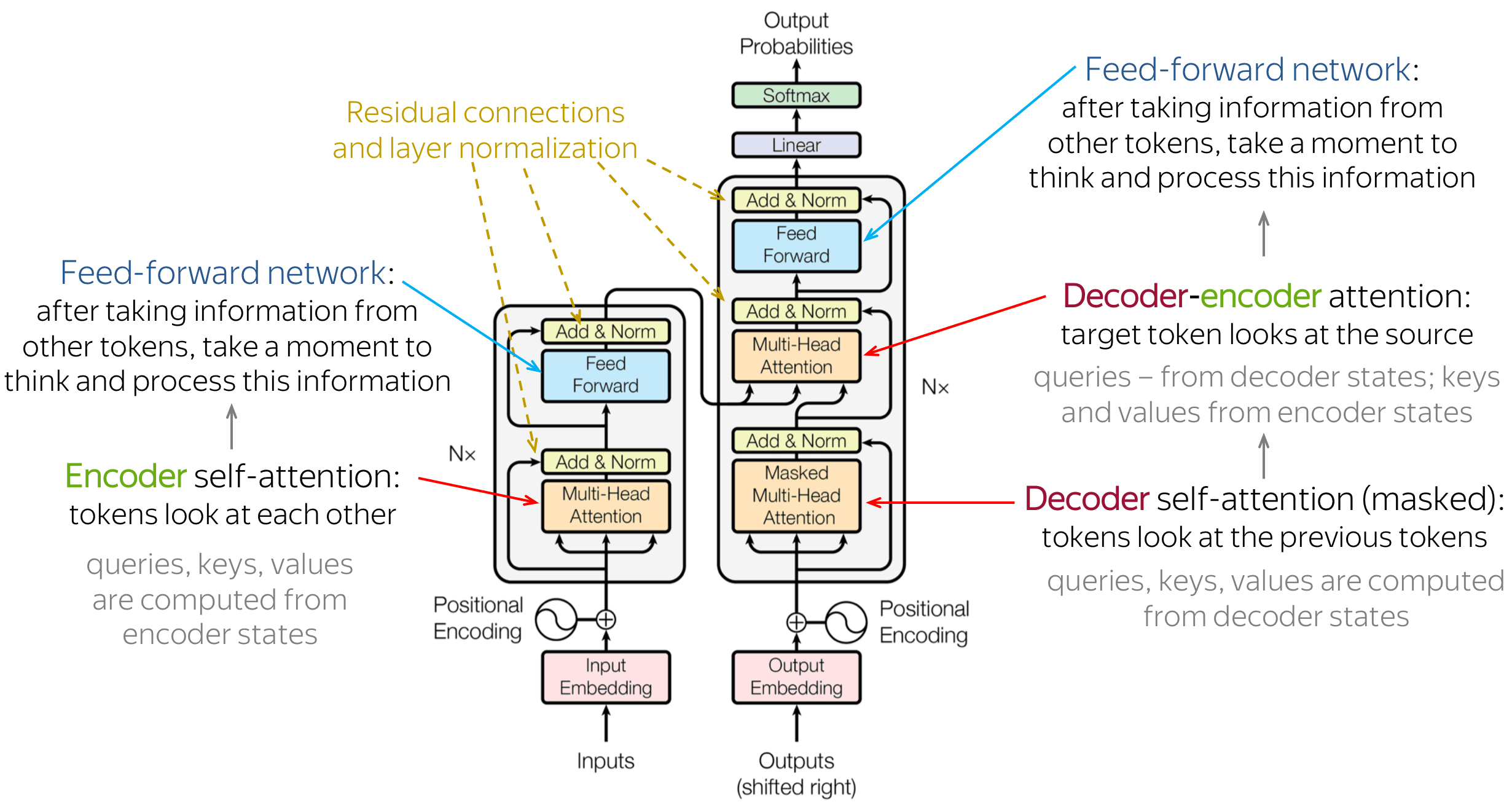
Transformer is the first transduction model relying entirely on self-attention to compute representations of its input and output without using sequence-aligned RNNs or convolution.
Transformer blocks are characterized by a multi-head self-attention mechanism, a position-wise feed-forward network, layer normalization modules and residual connectors.
- Transformer结构及其应用--GPT、BERT、MT-DNN、GPT-2 - 知乎
- 放弃幻想,全面拥抱Transformer:自然语言处理三大特征抽取器(CNN/RNN/TF)比较
- The Illustrated Transformer
- The Illustrated BERT, ELMo, and co. (How NLP Cracked Transfer Learning)
- Universal Transformers
- Understanding and Improving Transformer From a Multi-Particle Dynamic System Point of View
- The Annotated Transformer
- A Survey of Long-Term Context in Transformers
- The Transformer Family
- https://www.idiap.ch/~katharas/
- https://arxiv.org/abs/1706.03762
- Superbloom: Bloom filter meets Transformer
- Evolution of Representations in the Transformer
- https://www.aclweb.org/anthology/2020.acl-main.385.pdf
- https://math.la.asu.edu/~prhahn/
- https://arxiv.org/pdf/1802.05751.pdf
- https://arxiv.org/pdf/1901.02860.pdf
- Spatial transformer networks
- https://lena-voita.github.io/nlp_course/seq2seq_and_attention.html
- Transformers are graph neural networks
- Transformers are RNNs: Fast Autoregressive Transformers with Linear Attention
- A Unified Understanding of Transformer's Attention via the Lens of Kernel
- https://github.com/tomohideshibata/BERT-related-papers
- https://github.com/google-research/bert
- https://pair-code.github.io/interpretability/bert-tree/
- https://arxiv.org/pdf/1810.04805.pdf
- https://arxiv.org/pdf/1906.02715.pdf
- BERT-is-All-You-Need
- Visualizing and Measuring the Geometry of BERT
- BertEmbedding
- https://pair-code.github.io/interpretability/bert-tree/
- https://zhuanlan.zhihu.com/p/70257427
- https://zhuanlan.zhihu.com/p/51413773
- MASS: Masked Sequence to Sequence Pre-training for Language Generation
- SenseBERT: Driving some sense into BERT
- https://github.com/clarkkev/attention-analysis
- https://keras.io/examples/nlp/masked_language_modeling/
- https://github.com/huanghonggit/Mask-Language-Model
- Probabilistically Masked Language Model Capable of Autoregressive Generation in Arbitrary Word Order
- https://www.aclweb.org/anthology/2020.acl-main.240/
- http://proceedings.mlr.press/v119/bao20a.html
- https://www.aclweb.org/anthology/D19-1633/
- Better Language Models and Their Implications
- https://github.com/openai/gpt-2
- https://openai.com/blog/tags/gpt-2/
- GPT‑3: Its Nature, Scope, Limits, and Consequences
- https://arxiv.org/abs/2005.14165
- https://www.sparkcognition.com/gpt-3-natural-language-processing/
- https://github.com/elyase/awesome-gpt3
- https://zhuanlan.zhihu.com/p/352350329
- https://openai.com/blog/image-gpt/
- https://github.com/openai/image-gpt
- Generative Pretraining from Pixels
- https://github.com/gupta-abhay/ViT
- https://abhaygupta.dev/blog/vision-transformer
- https://arxiv.org/abs/2012.12556v3
- Structured State Spaces: A Brief Survey of Related Models
- https://github.com/state-spaces/mamba
- https://paperswithcode.com/search?q=author%3AAlbert+Gu&order_by=stars
- https://arxiv.org/pdf/2003.08271.pdf
- https://github.com/onnx/models
- https://www.zhihu.com/question/449261221
- https://openai.com/blog/
- https://github.com/facebookresearch/llama
- https://github.com/ggerganov/llama.cpp
- https://awinml.github.io/llm-ggml-python/
- https://llama-2.ai/
- https://www.llamaindex.ai/
- https://lorenlugosch.github.io/posts/2020/07/predictive-coding/
- https://github.com/miyosuda/predictive_coding
- https://huggingface.co/transformers/
- https://github.com/huggingface/transformers
- https://github.com/facebookresearch/ParlAI
DeepSpeed is a deep learning optimization library that makes distributed training easy, efficient, and effective.
- Applied Natural Language Processing
- HanLP:面向生产环境的自然语言处理工具包
- Topics in Natural Language Processing (202-2-5381) Fall 2018
- CS 124: From Languages to Information Winter 2019 Dan Jurafsky
- CS224U: Natural Language Understanding
- CS224n: Natural Language Processing with Deep Learning
- CS224d: Deep Learning for Natural Language Processing
- CS224n: Natural Language Processing with Deep Learning, Stanford / Winter 2019
- Deep Learning for NLP