Project Repository Link --> https://github.com/SGNovice/Disease-detection-using-chest-xrays/
The project utilizes a new chest X-ray database, namely “ChestX-ray8”, to build a lung disease detection system. The ChestX-ray8 comprises 108,948 frontal view X-ray images of 32,717 unique patients, and 14 disease labels which had been text-mined from associated radiological reports using natural language processing.
Chest X-Rays are considerably reliable radiobiological imprints of patients, which are widely used to diagnose an array of common diseases affecting organs within the chest. For too long, vast accumulations of image data and their associated diagnoses have been stored in the Picture Archiving and Communication Systems (PACS) of several hospitals and medical institutions. Meanwhile, data-hungry deep learning systems lie in wait of voluminous databases like these, at the cusp of fulfilling the promise of automated and accurate disease diagnosis. Through this project, we hope to unite one such vast database, the “ChestX-ray8" dataset, with a powerful deep Learning system, and automate the diagnosis of 14 common lung conditions. For this project phase, we focus on detecting three conditions - Cardiomegaly, Effusion, Emphysema - in addition to healthy states.
Deep learning, also known as hierarchical learning or deep structured learning, is a type of machine learning that uses a layered algorithmic architecture to analyze data. Unlike other types of machine learning, deep learning has an added advantage of being able to make decisions with significantly less human intervention. While basic machine learning requires a programmer to identify whether a conclusion is correct or not, deep learning can gauge the accuracy of its answers on its own due to the nature of its multi-layered structure. The emergence of modern frameworks like PyTorch, has also made preprocessing of data more convenient. Many of the filtering and normalization tasks that would involve a lot of manual tasks while using other machine learning techniques, are taken up automatically.
The essential characteristics of deep learning make it an ideal tool for giving the much needed impetus, to the field of automated medical diagnosis. With the right expertise, it can be leveraged to overcome several limitations of conventional diagnosis done by medical practitioners, and take the dream of accurate and efficient automated disease diagnosis to the realm of reality.
Given the team's vision to make healthcare better for everyone, everywhere, and having paid attention to the trends and recent breakthroughs with deep learning, we decided to experiment with several variations of convolutional neural networks for this project. Recent work has shown that convolutional networks can be substantially deeper, more accurate, and efficient to train if they contain shorter connections between layers close to the input and output. We embraced this observation, and leveraged the power of the Dense Convolutional Network (DenseNet), which connects each layer to every other layer in a feed-forward fashion. Whereas traditional convolutional networks with L layers have L connections - one between each layer and its subsequent layer - our network had L(L+1)/2 direct connections. We also experimented with other architectures, including residual networks, and used our model variations as controls to validate each other.
Convolutional Neural Networks are inherently designed for image processing, and this sets them up for handling and gathering insights from large images more efficiently.
Currently, some CNNs have approached, and even surpassed, the accuracy of human diagnosticians in identifying important features, according to a number of diagnostic imaging studies. In June of 2018, a study in the Annals of Oncology showed that a convolutional neural network trained to analyze dermatology images identified melanoma with ten percent more specificity than medical practitioners.Additionally, researchers at the Mount Sinai Icahn School of Medicine have developed a deep neural network capable of diagnosing crucial neurological conditions, such as stroke and brain hemorrhage, 150 times faster than human radiologists. The tool took just 1.2 seconds to process the image, analyze its contents, and alert providers of a problematic clinical finding.
Evidently, there is great potential for the future of healthcare with smart tools which integrate deep learning.
Among the several benefits artificial intelligence promises to bring to healthcare, these are worth highlighting.
- More affordable treatment: Diagnosis is faster and more accurate with automation; doctors will be able to recommend the right treatments to patients or intervene appropriately before illnesses aggravate leading to more expensive treatment options.
- Safer solutions: More accurate diagnosis means there will be a lower risk of complications associated with patients receiving ineffective or incorrect treatment.
- More patients treated: A reduction in the time it takes to complete a diagnostic analyses means laboratories can perform more tests. This will lead to coverage for more patients within shorter duration.
- Addressing the global ‘Physician Shortage’: The growing deficit between the demand for physicians and the supply, has been a growing concern for many countries around the world. The World Health Organization (WHO) estimates that there is a global shortage of 4.3 million physicians, nurses, and other health professionals. The shortage is often starkest in developing nations due to the limited numbers and capacity of medical schools in these countries. Additionally, these nations have many more rural and remote areas, which complicates the issue with other challenges like lack of good transportation. The growing need for more qualified medical personnel worldwide is like an incomplete jigsaw puzzle; training human personnel is expensive and will take significant amount of time to meet the demand. Automation with deep learning systems provide a comparably faster, scalable and a comparably low cost complement for salvaging the situation.
There is no denying the fact that with an ever-growing global population, we are going to need alternative AI-based medical personnel to assist us in achieving the sustainable development goal of providing “Affordable, Accurate and Adequate Healthcare for All”.
This project is borne out of the team's vision to make healthcare better for everyone, anywhere.
Given our time constraint, we chose to divide ourselves into sub-teams corresponding to the demarcated phases of this project. The benefit of this approach was a smooth iterative process - where we could have quick adjustments from previous phases to facilitate better outcomes for a subsequent phase - and speed due to parallel implementations at the various phases. We also adopted a scrum model, where the entire period was a sprint, and stand-up sessions within 2-day intervals served for progress updates and team re-orientation where it was necessitated. Finally, our team model allowed us to use initial cycles as an exploration to inform our final data selection and preprocessing, and model strategies. With each cycle, we redefined our goals while maintaining the general objective of facilitating faster lung X-ray assessments.

The dataset was highly imbalanced; the highest and lowest class counts were 60,361 and 110 respectively. It was also huge for our timeline, and we had to derive a better-balanced sample. We initially scaled down from 112,000+ images to 11,000+, and then eventually 8,186.
We also focused on images with single conditions, discarding images which showed multiple conditions and, therefore, had multiple class labels.
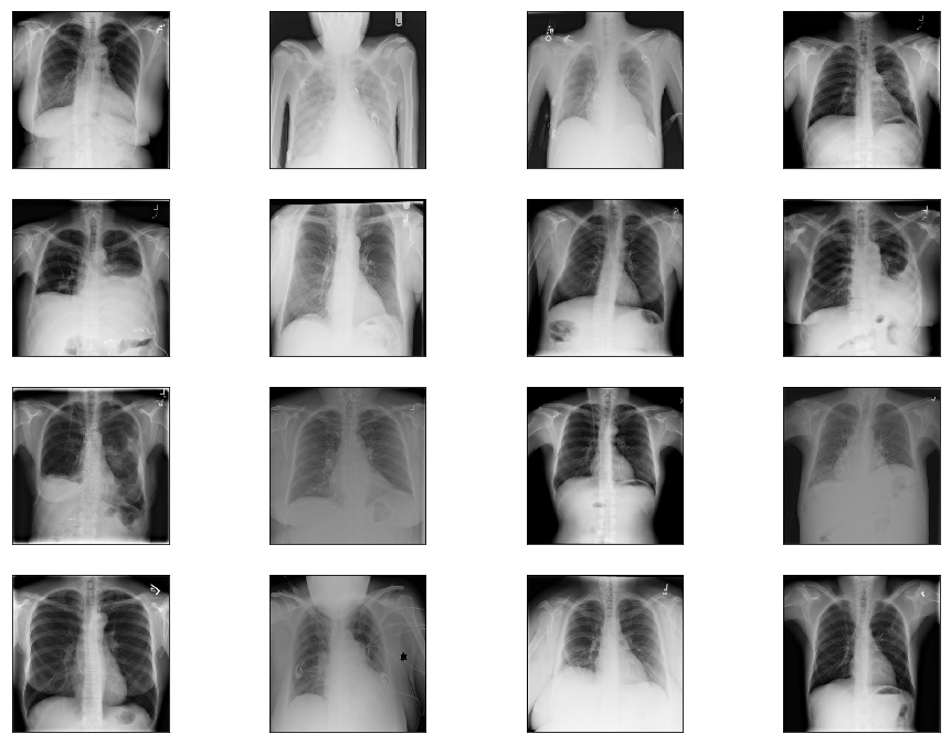
Sample images from the original dataset are shown below:
The initial distribution for images with single class labels is given below.
| Labels | Distributions |
|---|---|
| No Finding | 60361 |
| Infiltration | 9547 |
| Atelectasis | 4215 |
| Effusion | 3955 |
| Nodule | 2705 |
| Pneumothorax | 2194 |
| Mass | 2139 |
| Consolidation | 1310 |
| Pleural_Thickening | 1126 |
| Cardiomegaly | 1093 |
| Emphysema | 892 |
| Fibrosis | 727 |
| Edema | 628 |
| Pneumonia | 322 |
| Hernia | 110 |
We initially tested our strategies for classifying all 15 conditions and redefined our goals through exploration, until in addition to identifying Healthy X-rays (No Finding), the model could more accurately classify two conditions: Cardiomegaly and Effusion.
For our final round, and based on clinical considerations, we proceeded with two sets:
- Version 4.1 - for images taken using both antero-posterior position (AP) and postero-anterior position (PA).
- Version 4.2 - containing images taken using PA for Effusion and healthy (No finding) classes, and AP and PA for cardiomegaly.
The exception was made for the latter due to inadequate PA images.
The distribution for Version 4.1 finally settled at:
- (AP + PA) Cardiomegaly – 1093
- (AP + PA) No Finding – 1500
- (AP + PA) Effusion - 1500
The distribution for Version 4.2 finally settled at:
- (AP + PA) Cardiomegaly – 1093
- (PA) No Finding – 1500
- (PA) Effusion - 1500
Our dataset covered medical conditions, the manifestations of which could be present at edges of X-ray images and we exercised caution with our transformations. After several deliberations and clinical considerations, we would avoid cropping and extreme random rotations and kept to these:
- Random Rotation: within the angle range -10 to 10, with expansion enabled
- Resize: to a size of 224 by 224 to match our densenet model input size
- Random Horizontal Flip
- Random Vertical Flip
- Conversion To Pytorch floatTensor type: This minimalistic approach was our shot at preserving as much information that would be clinically relevant for diagnosing our target conditions.
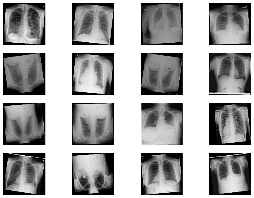
Sample images from the transformed dataset are as below:
The modeling stage was characterized by several iterative cycles that called for new sampling and processing strategies on demand. Notwithstanding, the team model facilitated swift responses so that we could re-orient quickly without disrupting overall progress. We also had the technical expertise that allowed us to try novel activation functions - namely mila, mish and beta mish – which we believe contributed greatly to our results.
Activation functions are important features of artificial neural networks. They determine whether a neuron should be activated or not; whether the information that a neuron is receiving is relevant for the given information or should be ignored.
It is an uni-parametric activation inspired by the Mish activation function - when β=1, β-Mish becomes the standard version of Mish - and can be mathematically represented using the function:

If β=1.5, the function ranges from ≈-0.451103 to ∞. For most benchmarks, β was set to be 1.5.

It is an uniparametric activation function inspired by the Mish Activation Function. The parameter β is used to control the concavity of the Global Minima of the Activation Function where β=0 is the baseline Mish Activation Function. Varying β in the negative scale reduces the concavity and vice versa. β is introduced to tackle gradient death scenarios due to the sharp global minima of Mish Activation Function.
The mathematical function of Mila is shown as below:

This activation function uses the square operator to introduce the required non-linearity as compared with the use of an exponential term in the popular TanSig. Smaller computational operation count characterizes the proposed activation function. The key to the effectiveness of this function is a faster convergence when used in Multilayer Perceptron Artificial Neural Network architectural problems. Additionally, the derivative of the function is linear, resulting in a quicker gradient computation.
ReLu Stands for Rectified Linear Unit. It is the most widely used activation function, and is chiefly implemented in hidden layers of neural networks.
- Equation :- A(x) = max(0,x). It gives an output x if x is positive and 0 otherwise.
- Value Range :- [0, inf]
- Nature :- Non-linear, which means we can easily backpropagate the errors and have multiple layers of neurons being activated by the ReLU function.
- Uses :- ReLu is less computationally expensive than tanh and sigmoid because it involves simpler mathematical operations. At a time, only a few neurons are activated making the network sparse, and computationally efficient.
The softmax function is also a type of sigmoid function but is handy when we are trying to handle classification problems.
- Nature :- non-linear
- Uses :- Usually used when trying to handle multiple classes. The softmax function would squeeze the outputs for each class between 0 and 1 and would also divide by the sum of the outputs.
- Output:- The softmax function is ideally used in the output layer of the classifier where we are actually trying to attain the probabilities to define the class of each input.
Deep Convolutional Neural Network (DCNN) architectures are favoured for weakly-supervised object localization for the advantages of large image capacity, various multi-label losses, and pooling strategies. In lieu of this, we experimented with the architectures outlined below, in a bid to explore and appreciate their suitability for this project.
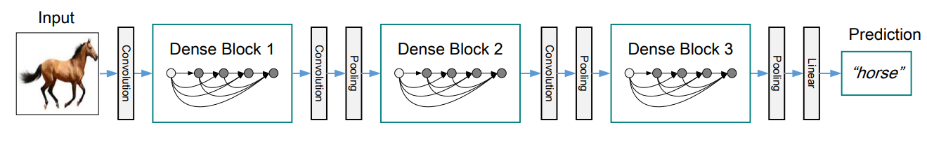
A DenseNet is a stack of dense blocks followed by transition layers.
Dense blocks consist of a series of units. Each unit packs two convolutions, each preceded by Batch Normalization and ReLU activations, and outputs a fixed-size feature vector. A parameter, described as the growth rate, controls how much new information the layers allow to pass through.
Transition layers, on the other hand, are very simple components designed to perform downsampling of the features passing through the network. Every transition layer consists of a Batch Normalization layer, followed by a 1x1 convolution, and then a 2x2 average pooling.
A deep residual network (deep ResNet) is a type of specialized neural network that helps to handle more sophisticated deep learning tasks, by facilitating better outcomes with deeper architectures. It has received growing attention in recent times, for its effectiveness for training deep networks. ResNet-50 is a 50-layer deep convolutional neural network that is pre-trained on more than one million images from the ImageNet database [1]. As a result, it has learned rich feature representations for a wide range of images, and can classify images into 1000 object categories.
One problem with deep networks composed of dozens of layers, as commonly cited by professionals, is that accuracy can become saturated, and some degradation can occur. Others are also concerned about the "vanishing gradient" problem, which is characterised by gradients becoming too small to be immediately useful. The other obvious reason is overfitting, where models learn intricate details from training data that prevent them from generalizing enough on unseen data.
The deep residual network deals with some of these problems by using residual blocks, which take advantage of residual mapping to preserve inputs. By utilizing deep residual learning frameworks, we could harness the power of deep networks and minimize the weaknesses.
ResNeXt is a simple, highly modularized network architecture for image classification. The network is constructed by repeating a building block that aggregates a set of transformations with the same topology. This simple design results in a homogeneous, multi-branch architecture that has only a few hyper-parameters to set. This strategy exposes a new dimension, which we call “cardinality” (the size of the set of transformations), as an essential factor in addition to the dimensions of depth and width.
Healthcare data is particularly sensitive, and we face the risk of exposing sensitive patient data through projects like ours. For ensuring security and privacy of the dataset, we implemented a class which would allow encryption of model and data on-demand using websockets and the PySyft library. A link to the our implementation is provided in the appendix of this document.
With varied approaches for data sampling, activation function selection and hyperparameter tuning, we trained and tested six models, codenamed Aurora, Ava, Auden, Venus, Armadillo, and Atlas. Our results are given below in descending order of model performance.
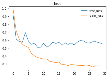
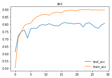
We trained and tested densenet161 with beta-mish and mila activations, on classifying Cardiomegaly, Effusion, and No Finding, irrespective of X-ray position using dataset version 4.2.
| Label | Accuracy |
|---|---|
| Cardiomegaly | 89.000% (89/100) |
| Effusion | 83.000% (83/100) |
| No Finding | 75.000% (75/100) |
| Overall | 82.3333% (247/300) |
Here are the graphs representing loss and accuracy for test and training dataset.
We trained and tested densenet161 with beta-mish and mila activations, on the dataset version 4.1 containing images for Cardiomegaly(mixed AP/PA), Effusion(PA), and No-Finding(PA)
| Label | Accuracy |
|---|---|
| Cardiomegaly | 83.000% (83/100) |
| Effusion | 79.000% (79/100) |
| No Finding | 76.000% (76/100) |
| Overall | 79.3333% (238/300) |
We trained and tested densenet161 with sqnl activation, on classifying Emphesyma and No-Finding, irrespective of X-ray position.
| Label | Accuracy |
|---|---|
| Emphysema | 70% (70/100) |
| No Finding | 80% (76/100) |
We trained and tested resnet50 with mila activation, on classifying Pneumothorax and No-Finding, irrespective of X-ray position.
| Label | Accuracy |
|---|---|
| Pneumothorax | 45% (45/100) |
| No Finding | 92% (92/100) |
We trained and tested densenet161 with mila activation on classifying Cardiomegaly, Effusion, and No-Finding, irrespective of X-ray position.
| Label | Accuracy |
|---|---|
| Cardiomegaly | 25% |
| Effusion | 80% |
| No Finding | 66% |
We trained and tested resNext50 with traditional ReLU and Softmax activations on classifying Cardiomegaly, Effusion, and No-Finding, irrespective of X-ray position.
Evidently, our most accurate model was AURORA, achieving an accuracy of 82.3%, on PA images for Effusion and Healthy X-rays(No-finding), and AP+PA images for cardiomegaly.
In comparison with similar work dedicated to lung disease detection using the same dataset we used, we have had better accuracies. There is a general appreciation of the difficulty of the task we gave ourselves in this project, and we recognise that we cleared a milestone that opens up many possibilities. We had our fair share of difficulties, notwithstanding. We ran into significant challenges in our attempt to find a working approach toward processing the Chest X-Ray dataset and training a successful deep learning model. While many factors can be taken into account for this complication, the root cause can be traced back to the original dataset itself. Some baseline imperfections posed challenges that had to be tackled by the Data Acquisition, Pre-processing and Modelling teams alike. We explore these challenges subsequently.
-
Chest X-Ray dataset was extremely imbalanced for the distribution of images for individual classes: For example, there was a huge disparity between the image counts for the top class(No Finding) with more than 60,000 and the bottom class(Hernia) with only 110.
-
X-ray images in our dataset were taken from two different positions: PA/posterior-anterior and AP/anterior-posterior: This especially held true for “Effusion” class, with the number of images captured in each position almost equal. Since many of the diseases in our dataset were sensitive to such positions, we were torn between splitting each class into two smaller ones - AP and PA - or more ideally, retaining only PA pictures.
The latter approach, nevertheless, had one major disadvantage: we needed to take into account the number of pictures in the PA position, which in many cases were not enough. Considering the limited number of PA images we had for “cardiomegaly”, we decided to include both PA and AP pictures in each class, and this would definitely have a negative impact on the accuracy of our model. -
Proceeding with data augmentation: Even a small rotation or central crop could result in loss of important diagnostic information and lead to inaacurate predictions. After extensive research on the dataset, the reported performance of past models, and several rounds of experimentation, we reduced the number of classes in the wrangled and modified dataset to only three - CardioMegaly, Effusion, and No finding. The sampled dataset became much more balanced and would prevent training bias.
-
X-ray images in the dataset were missing some crucial information typically used for diagnosing diseases: After consulting with the subject matter expert in our team, we found that for conditions that tend to look similar in X-ray images such as “Mass”, “Infiltration” and “Pneumonia”, in real life doctors would rely on other factors such as white count and temperature to make a formal diagnosis. Unfortunately, that information was not available in our dataset. In fact, in the original paper, all the aforementioned diseases performed poorly and recorded a high prediction error rate from the model, which helped to reinforce our earlier finding. We would resort to focusing of xray samples of distinct conditions.
-
Disease labels for the X-ray chest dataset were not done manually, but rather through a number of different NLP techniques when constructing the image database: Although the authors had gone the extra mile in mitigating the risk of wrong labeling, by crafting a variety of custom rules and then applying them in the pre-processing step, the problem of defective labels was not entirely eliminated. Specifically, we can refer to “Table 2. Evaluation of image labeling results on OpenI dataset.” on page 4 of the paper for a detailed assessment on this phenomenon. The vast majority of classes exhibited varying degrees of being mislabeled, from "Effusion" with 0.93 precision rate, to "Infiltration" with a modest score of 0.74. Owing to this imperfection, our models had a baseline limitation on how accurate they could become.
-
Ignoring the fourth channel: The original image data had an extra alpha(transparency) channel, which is supposed to help with the assessment of manifestations of some conditions. Due to the constraints of compute resources, however, we had to reduce the channels to three, to reduce the computational cost. This may have contirbuted to some inaccurate classifications.
Our project adds emphasis to the immense potential to be harnessed from the intersection of Deep Learning and Medical Diagnostics. The outcomes achieved within the short span of time were commendable. We also appreciated the technicalities of medical imaging, and more importantly, the challenges with automated diagnosis leveraging analysis of x-ray images by deep neural networks. Our goal is to build a full system that leverages federated learning and full blown secure and privacy preserving technologies, to make smart diagnosis accessible in the browser, on phones and tablets - the web interface is up and functional, while the mobile platforms are underway. We have also designed a roadmap which will allow us to improve the overall quality and accuracy of our system on available datasets for chest X-rays. Ultimately, we hope to build on this project for other diagnoses outside our current target of 14 lung conditions.
The team would like to extend the project to make it suitable for use in institutions and facilities, where aid to diagnosis is of utmost importance.
Currently, the project is limited to the public domain dataset and to the best-effort analyses of health records via natural language processing. The idea here is to improve the current accuracy of the model by augmenting it with real-world datasets which are available from medical institutions. Due to the sensitive nature of these datasets and concerns for privacy, these are currently being kept private. With the power of federated learning, we can adopt a strategy where medical institutions would not need to relent their private datasets to a central server, which might lead to privacy leakage. Instead, we open an interface for them to feed the data within the institution, train the model on-site and only transmit gradients and other model information to the central server which we have access and do model aggregation accordingly. Firstly, we will coordinate with medical institutions to install Internet-enabled devices on-premise. For this, we think of Raspberry Pi 3 devices, small, lightweight and powerful enough to perform the local training needed. We plan on creating a headless setup to each Raspberry Pi device, with the web server connected to their local network. This web server can be accessed by representatives in-house to feed X-ray data and other relevant information pertinent to local training. We make sure that the data to be fed locally matches the global requirements for model improvement. We can send the model definition to each Raspberry Pi’s installed remotely. We then orchestrate model updates on-demand using the power of PySyft’s secure model parameter aggregation, leveraging mathematical techniques per actor to encrypt model information so trusted aggregators cannot glean on raw gradients sent by federated nodes. We will need the full cooperation of hospitals, clinics and radiologic facilities who have quality datasets to join our planned IoT-enabled ecosystem for this use case. In return, we will enable an intuitive interface to help doctors in diagnosis.
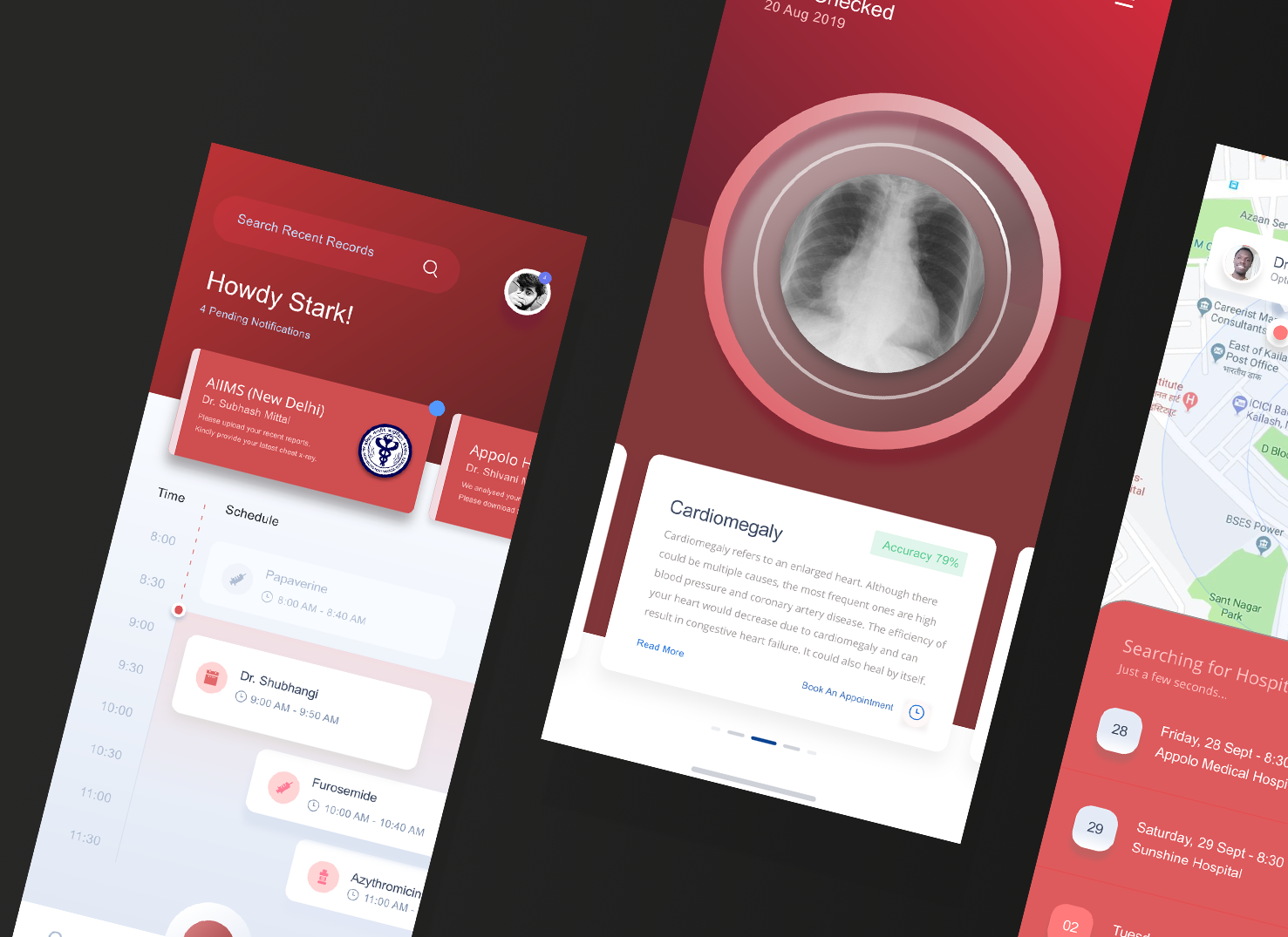
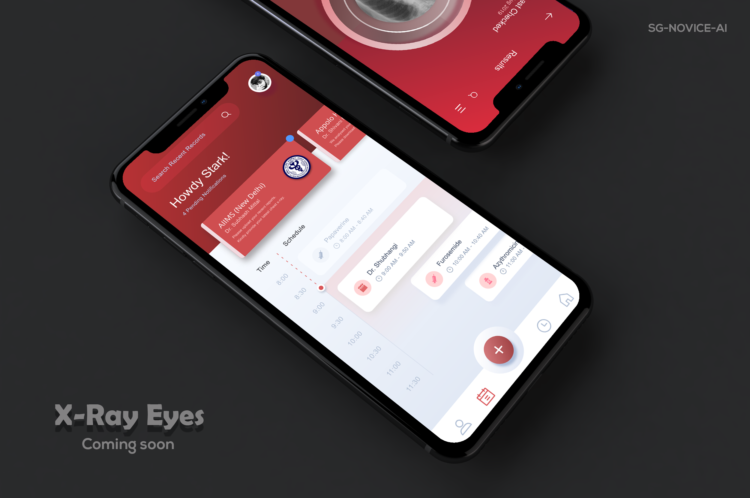
We already deployed the model to the web for demonstration, and our xray detection service is accessible at https://xrayeyes.onrender.com. We have also started work on the apps for android, iOS and the new ipadOS. Additionally, these mobile apps may be used in the home, and we have designed functionality that can link patients to nearby clinics or hospitals. Mocks of this is shown below:
- Data Exploration Notebook https://colab.research.google.com/drive/1nub56-UfvlovgWP7oSC5850HdNIbOFQu
- Model Encryptor https://github.com/ayivima/AI-SURFS/blob/master/ModelEncryptor/encryptor.py
- Mobile Platform UI Mocks (a)https://raw.githubusercontent.com/SGNovice/Disease-detection-using-chest-xrays/master/images/xrayeyes2.png (b)https://raw.githubusercontent.com/SGNovice/Disease-detection-using-chest-xrays/master/images/xrayeyes.png
- XrayEyes Web App Demo https://xrayeyes.onrender.com
| Members | GitHub Handle |
|---|---|
| Victor Mawusi Ayi | https://github.com/ayivima |
| Anju Mercian | https://github.com/amalphonse |
| George Christopoulos | https://github.com/geochri |
| Ashish Bairwa | https://github.com/ashishbairwa |
| Pooja Vinod | https://github.com/poojavinod100 |
| Ingus Terbets | https://github.com/ingus-t |
| Alexander Villasoto | https://github.com/anvillasoto |
| Olivia Milgrom | https://github.com/OliviaMil |
| Tuan Hung Truong | https://github.com/tuanhung94 |
| Marwa Qabeel | https://github.com/MarwaQabeel |
| Shudipto Trafder | http://github.com/iamsdt |
| Aarthi Alagammai | https://github.com/AarthiAlagammai |
| Agata | https://github.com/agatagruza |
| Kapil Chandorikar | https://github.com/kapilchandorikar/ |
| Archit | https://github.com/gargarchit |
| Cibaca Khandelwal | https://github.com/cibaca |
| Oudarjya Sen Sarma | https://github.com/oudarjya718 |
| Rosa Paccotacya | https://github.com/RosePY |
https://arxiv.org/pdf/1705.02315.pdf
https://www.kaggle.com/ingusterbets/nih-chest-x-rays-analysis
https://github.com/digantamisra98/Mila
https://github.com/digantamisra98/Beta-Mish
https://nihcc.app.box.com/v/ChestXray-NIHCC/folder/37178474737
https://nihcc.app.box.com/v/ChestXray-NIHCC/file/219760887468
https://link.springer.com/chapter/10.1007/978-3-540-75402-2_4