3. Tutorials
Open the file alpss_run.py. In the file there is a docstring that describes the input variables followed by the function alpss_main. No input parameters need to be changed from the original repository file to run the demo. The program will run the example file in the input_data folder.
In the alpss_run file there is a section that reads
# %%
from alpss_main import *
import os
Just above these lines there should be small font options that read "Run Cell | Run Below | Debug Cell" (see image below). Click the "Run Cell" button and the program will execute in an interactive notebook window. Note that this "Run Cell" option is only available through VS Code with the Jupyter extension, which is the recommended method.

Additional example data files are available through the paper by DiMarco et al. and can be accessed here.
Instructions on how to run your own data can be found in the repository wiki here. The final output plots should look like this:

- Move example_file.csv out of the input_data directory and into some other temporary directory of your choosing. It does not matter where this temporary directory is located on your machine.
- Open the alpss_auto_run.py file and click "Run Cell", similar to the example above. This will open an interactive notebook and the program will execute. The program is now waiting for a file to be moved into the directory that it is monitoring, the input_data directory.
- Click and drag example_file.csv out of your temporary directory and into the input_data directory. The program will automatically detect that a file has been added and run it through the ALPSS program.
The output figure should be the same as above.
When importing your own data there are several variables that HAVE TO BE adjusted to properly read in the file. These variables are listed below. Be especially careful when setting time_to_skip, time_to_take, t_before, and t_after. If these variable are set incorrectly an error may be thrown because the code can end up trying to analyze a section of time that hasn't actually been imported.
-
filename
- Indicates the name of the file you want to import.
-
start_time_user
- If input as 'none' ALPSS will attempt to automatically find the signal start time. If you wish to manually input a signal start time simply replace 'none' with a float that indicates the start time of the signal in the imported data.
-
header_lines
- Indicates the number of header lines in your input file.
-
time_to_skip
- Indicates the the amount of time you wish to skip in the original data file before any data is read in to the program. For example, if the full data file is 20 microseconds but the signal doesn't start until around 10 microseconds, time_to_skip can be input as 9e-6 to tell the program to ignore the first 9 microseconds of data. It is important to leave a buffer in the imported data before the signal actually starts to allow the program to accurately locate the carrier band.
-
time_to_take
- Indicates the amount of time you wish to read in from the original data file. For example, if the full data file is 20 microseconds but you only want to read in 2 microseconds of data, time_to_take should be changed to 2e-6.
-
t_before
- Indicates the amount of time from before the signal start time that will be included in the region of interest.
-
t_after
- Indicates the amount of time from after the signal start time that will be included in the region of interest. It is important to ensure that t_after will not extend the region of interest past the the amount of time that originally imported from the data file. This will result in an error if input incorrectly.
-
freq_min
- Indicates the upper frequency bound of the region of interest and band pass filter. All frequency powers above this level will be zeroed out.
-
freq_max
- Indicates the lower frequency bound of the region of interest and band pass filter. All frequency powers below this level will be zeroed out. It is important to select a lower bound that leaves a buffer to the carrier band to allow for accurate calculation of the carrier band and carrier frequency.
-
sample_rate
- Indicates the sample rate of the oscilloscope used to collect the data.
-
exp_data_dir
- Indicates the directory that the experimental data file is stored in.
-
out_files_dir
- Indicates the directory that the output data files will be saved to.
The user input start_time_correction allows the user to input a correction that will be added to the detected signal start time. Using the sample file change the input start_time_correction from 0e-9 to 4e-9 to get the following result:

In the Thresholded Spectrogram sub plot you now see a dashed red line and a solid red line. The dashed line represents the start time that ALPSS originally detected and the solid line represents the detected start time with the correction added in. The new corrected start time is where ALPSS will begin to filter the carrier frequency as seen in the sub plot Filtered Spectrogram ROI. Also notice how changing the signal start time changes the velocity profile early in the signal during the rise. Caution must be taken here as this can sometimes produce a signal that falsely looks like it has an HEL (Hugoniot Elastic Limit) but is really just noise.
The user can also override the automatic ROI finder by inputting a hard coded start time in the variable start_time_user. Setting start_time_correction to 0 and changing start_time_user to 620e-9 produces the following result. Notice how the signal start time is now marked exactly at the user input value of 620ns and how the shape of the velocity rise changes compared to the first example. The velocity signal is sticking a bit to the carrier frequency and not correctly picking up the beginning of the velocity rise.

The problem of changing the shape of the velocity rise depending on the signal start time can be mitigated with adjustments to the carrier filter. Keeping start_time_user at 620e-9, change wid to 2e8 to get the following result. Again, observe the change to the early signal rise. The carrier signal has now been more strongly filtered (starting after the signal start time), so the velocity more accurately follows the initial rise instead of sticking to the carrier.

Once ALPSS has chosen a signal start time the time domain of interest is selected based on the user inputs t_before and t_after, which specify the amount of time before the signal start time to take and the amount of time after the signal start time to take. For example, starting with the input parameters the same as in the original repository file, changing t_before to 12e-9 and t_after to 100e-9 gives the following result:

The frequency range for the region of interest (ROI) is set by the user prior to the run in the variables freq_min and freq_max. Starting with the input parameters the same as in the original repository file, changing freq_min to 0.5e9 and freq_max to 5e9 gives the following result:

The user should try to keep the frequency range tight to the signal, as extending the frequency range increases the chance that high power random noise will incorrectly be chosen as the signal start time.
Starting after the signal start time, the carrier frequency is filtered out using a Gaussian notch with the input parameters order and wid which adjust the order and width of the Gaussian notch, respectively. Using the original inputs and changing order=6 and wid=1e8 we get:

But if we change the inputs to order=6 and wid=5e5 we get:

Notice how the thinner width of the notch fails to adequately reduce the power of the carrier after the signal start time. This results in the velocity trace being pulled down to the zero velocity carrier instead of remaining on the true signal.
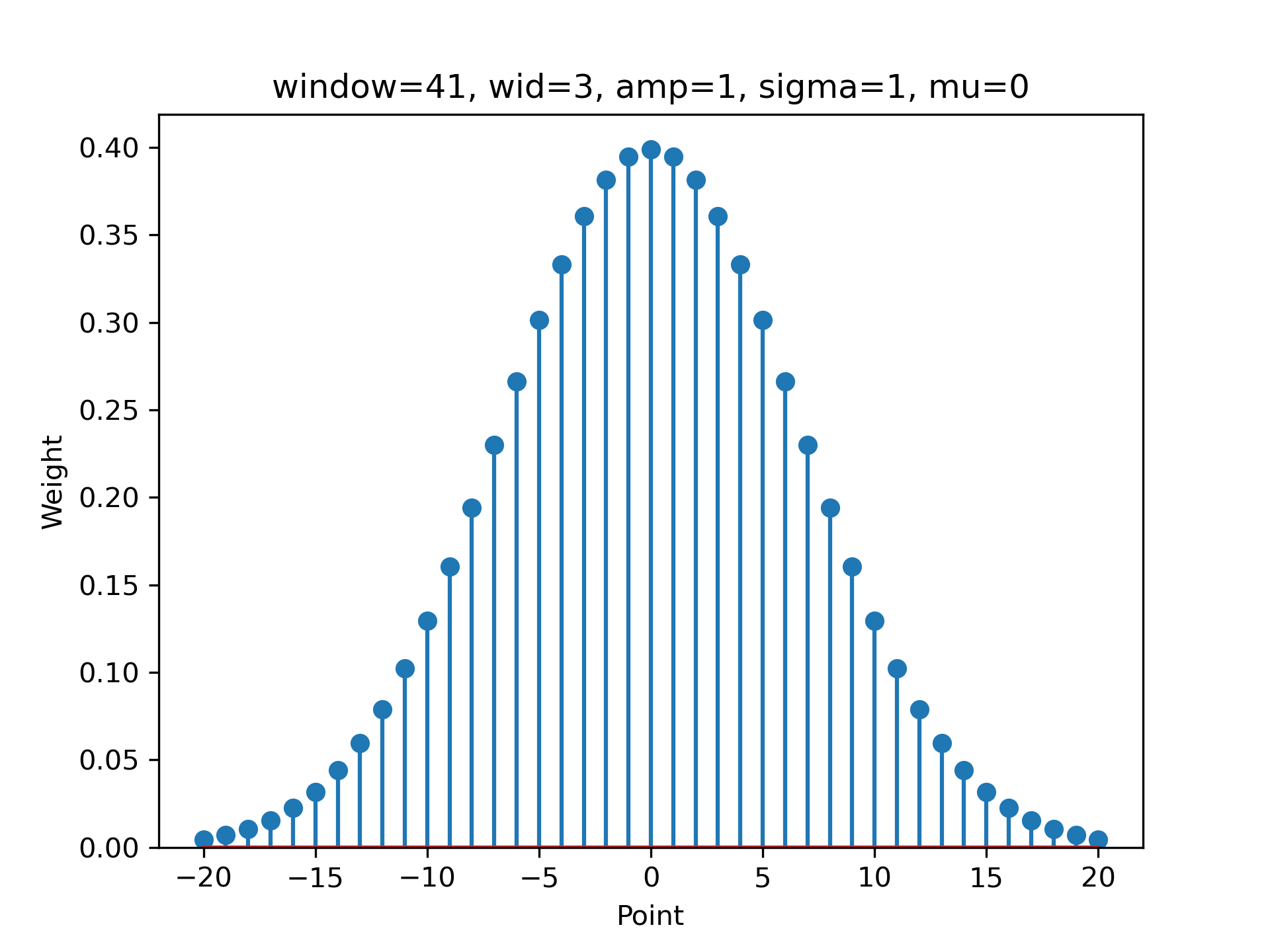
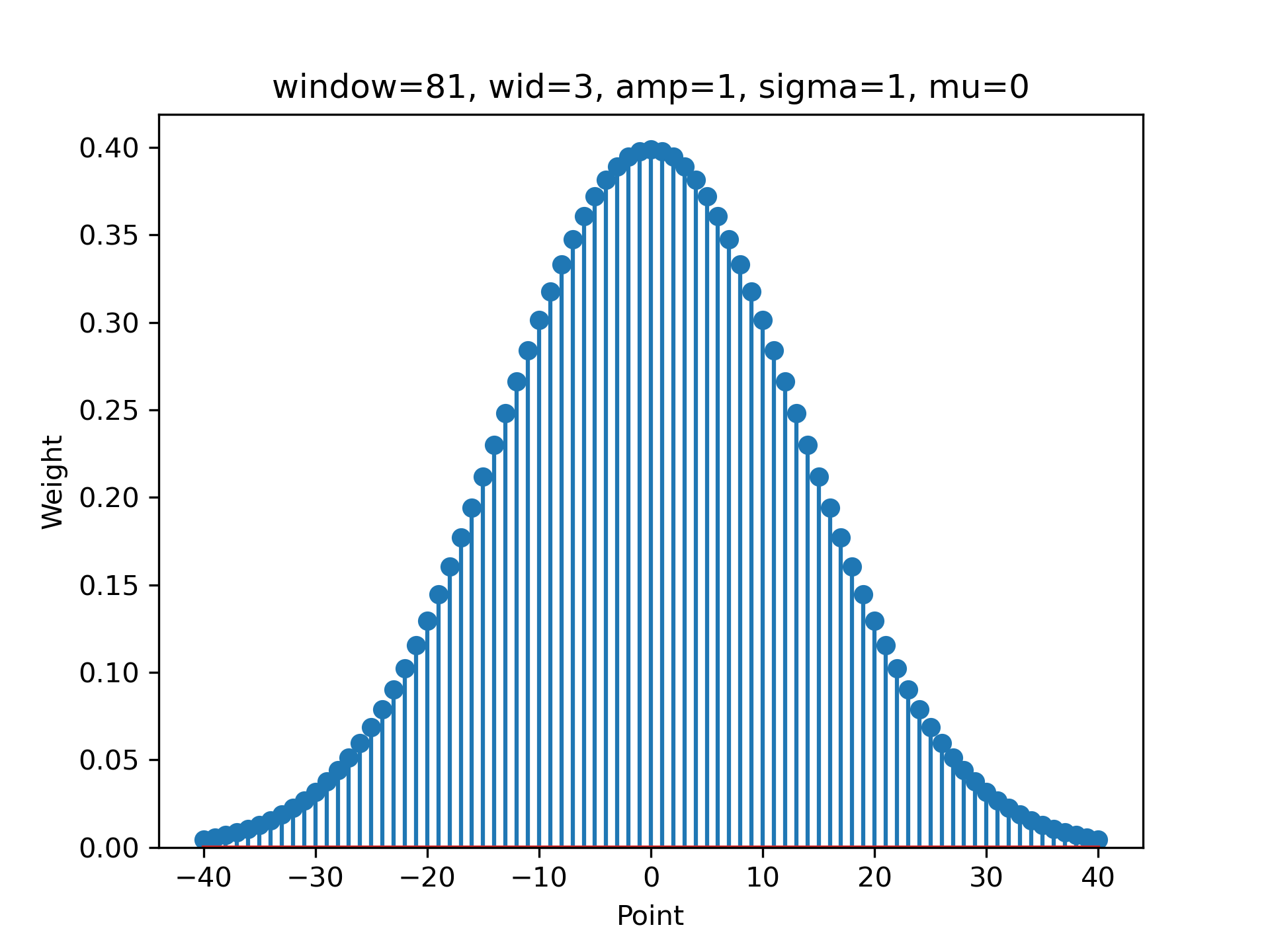
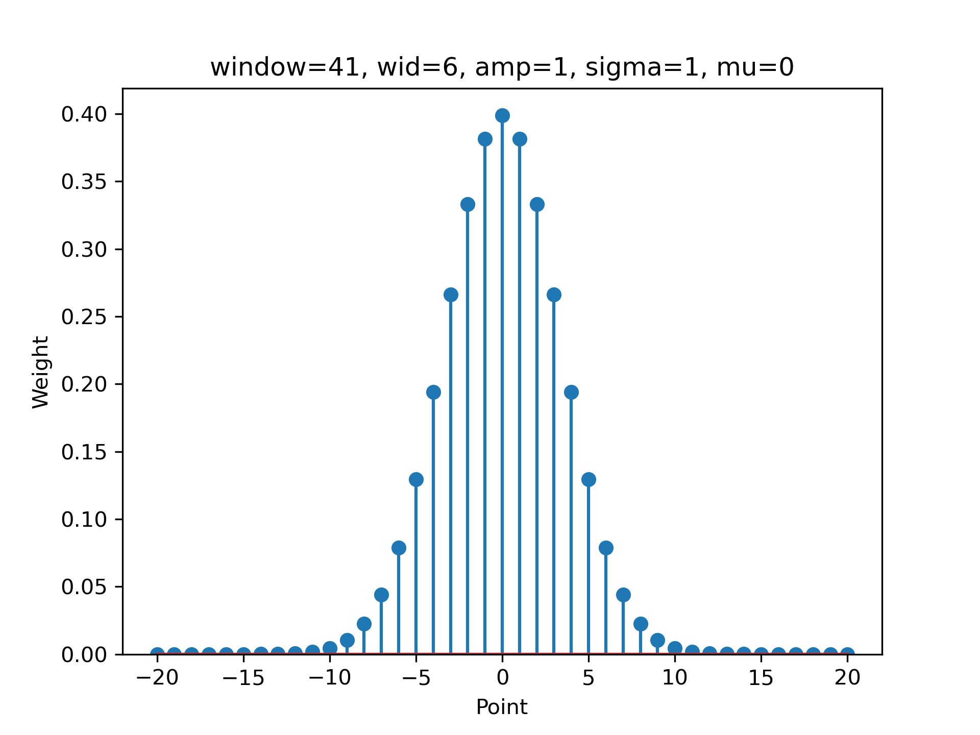
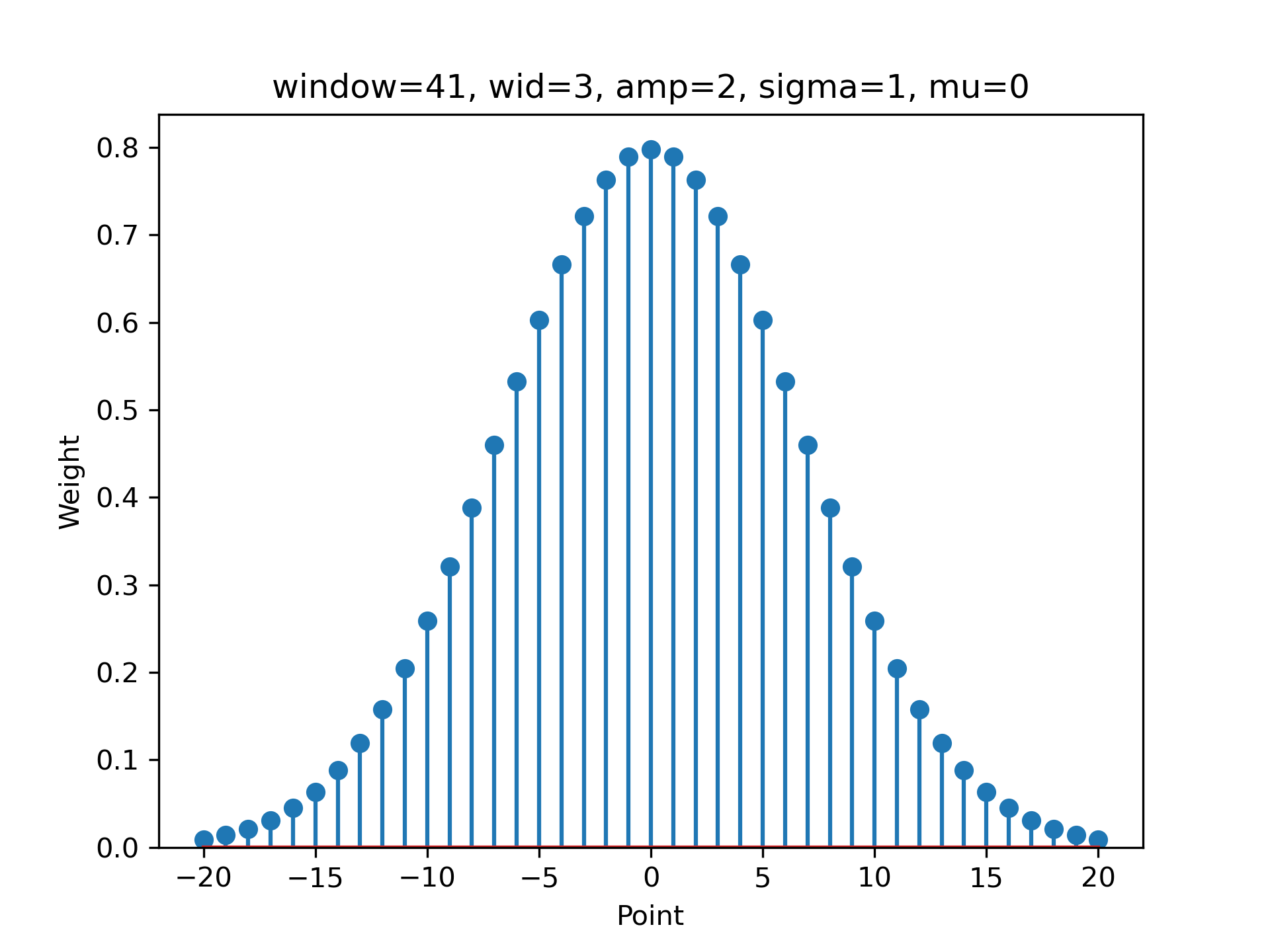
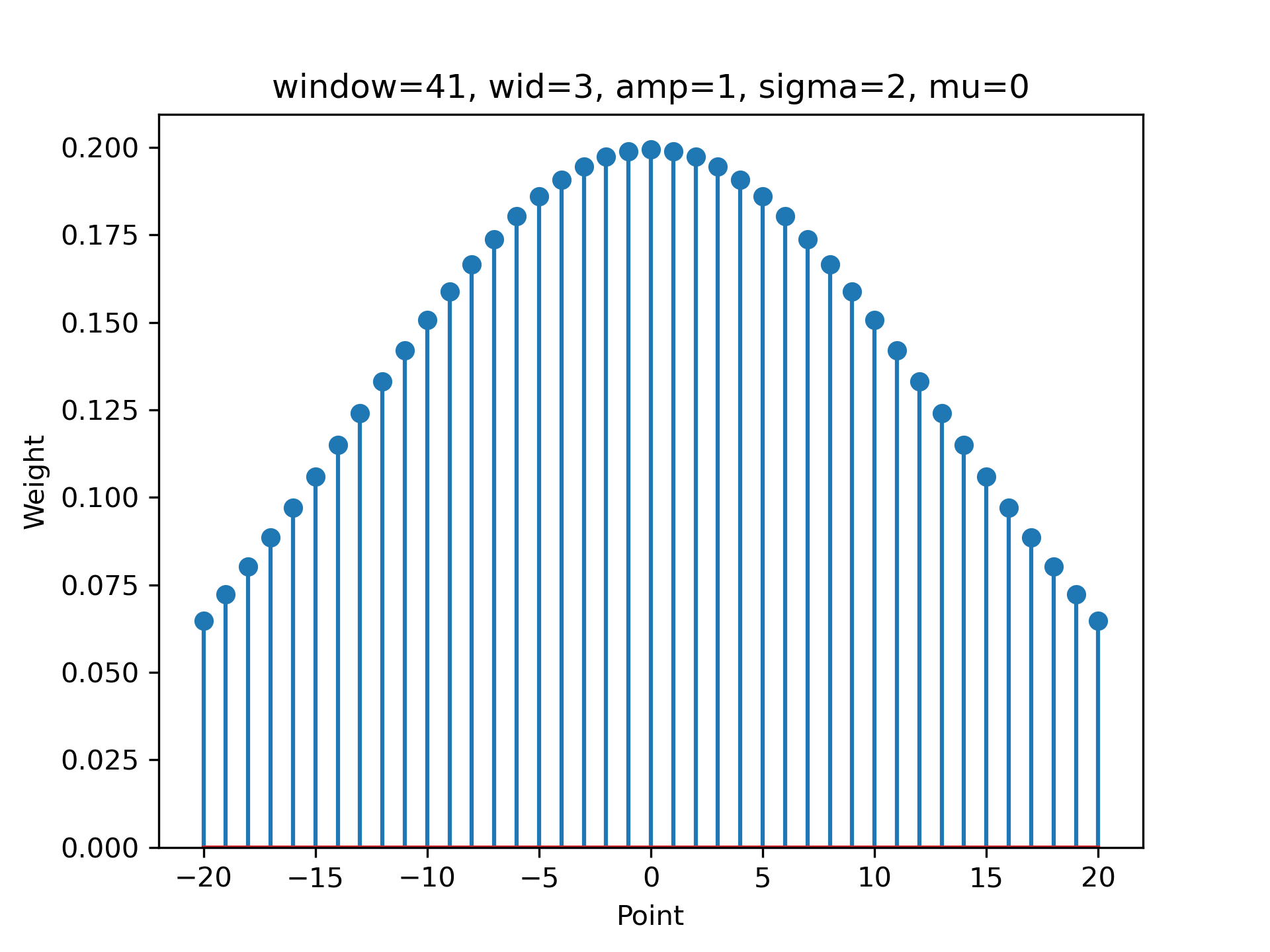
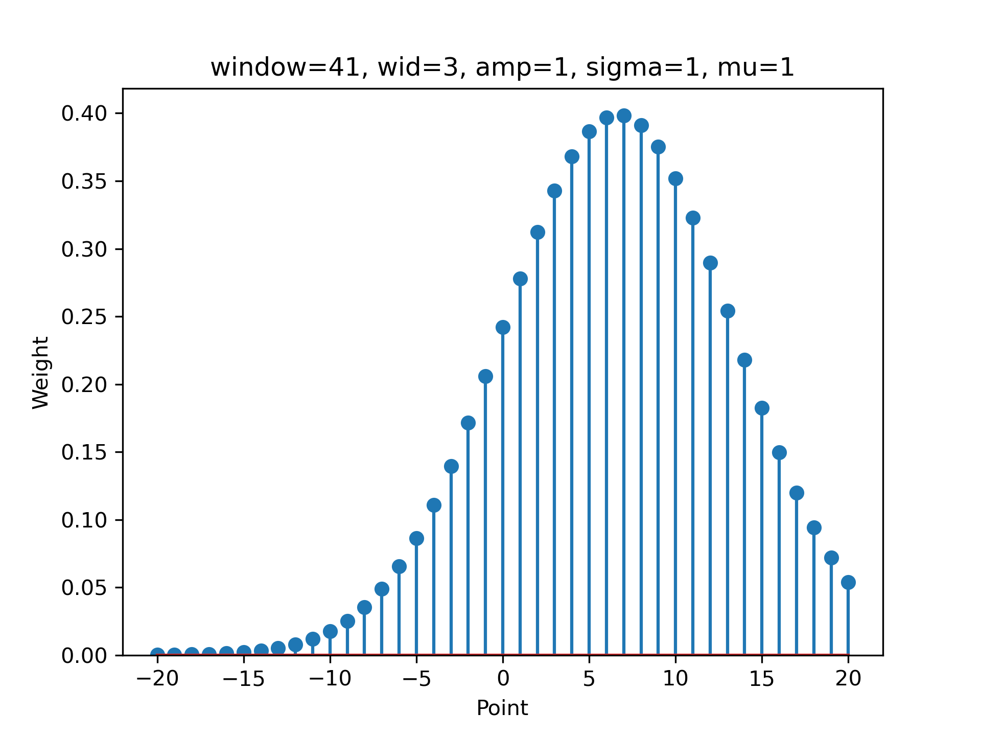
Smoothing of the velocity signal is accomplished using a Gaussian weighted moving average. The parameters of the Gaussian distribution that the weights are calculated from are input in the variables smoothing_window, smoothing_wid, smoothing_amp, smoothing_sigma, and _smoothing_mu, which are the number of smoothing points, the width of the Gaussian distribution, the amplitude of the Gaussian distribution, the standard deviation of the Gaussian distribution, and the mean of the Gaussian distribution. The following plots show the effects of these input parameters on the smoothing weights.
After the velocity trace has been calculated, ALPSS attempts to locate three separate local extrema.
- The point at which the sample undergoes maximum compression (the global maximum of the velocity trace)
- The point at which the sample undergoes maximum tension (the local minimum following the global maximum)
- The point at which the sample undergoes recompression (the local maximum following the max tension local minimum)
These points are located using rudimentary peak finding by comparing to a certain number of neighboring points. The number of neighboring points to compare to can be adjusted for the tension and recompression points and are specified in the inputs pb_neighbors and rc_neighbors, respectively. For example in the following plot pb_neighbors and rc_neighbors are both set to 200.

But if pb_neighbors and rc_neighbors are both changed to 600 we get:

Which local extrema are selected can also be changed using the inputs pb_idx_correction and rc_idx_correction. Instead of changing the number of neighbors these inputs change which peak is selected. For example if pb_neighbors and rc_neighbors are both set back to 200 but now pb_idx_correction and rc_idx_correction are both changed from 0 to 1 we get:

This works by selecting the second local minimum and maximum after the global maximum instead of taking the first local minimum and maximum after the global maximum.