Included Packages

penaltymodel
penaltymodel-cache
penaltymodel-maxgap
penaltymodel-mip
penaltymodel-lp

penaltymodel

One approach to solve a constraint satisfaction problem (CSP) using an Ising model or a QUBO, is to map each individual constraint in the CSP to a 'small' Ising model or QUBO. This mapping is called a penalty model.

Imagine that we want to map an AND clause to a QUBO. In other words, we want the solutions to the QUBO (the solutions that minimize the energy) to be exactly the valid configurations of an AND gate. Let z = AND(x_1, x_2).

Before anything else, let's import that package we will need.

import penaltymodel.core as pm
import dimod
import networkx as nx

Next, we need to determine the feasible configurations that we wish to target (by making the energy of these configuration in the binary quadratic low). Below is the truth table representing an AND clause.

AND Gate

x_1	x_2	z
0	0	0
0	1	0
1	0	0
1	1	1

The rows of the truth table are exactly the feasible configurations.

feasible_configurations = {(0, 0, 0), (0, 1, 0), (1, 0, 0), (1, 1, 1)}

We also need a target graph and to label the decision variables. We create a node in the graph for each variable in the problem, and we add an edge between each node, represnting the interactions between the variables. In this case we allow an interaction between every variable, but more sparse interactions are possible. The labels of the nodes and the decision variables match.

graph = nx.Graph()
graph.add_edges_from([('x1', 'x2'), ('x1', 'z'), ('x2', 'z')])
decision_variables = ['x1', 'x2', 'z']

We now have everything needed to build our Specification. We have binary variables so we select the appropriate variable type.

spec = pm.Specification(graph, decision_variables, feasible_configurations, dimod.BINARY)

At this point, if we have any factories installed, we could use the factory interface to get an appropriate penalty model for our specification.

p_model = pm.get_penalty_model(spec)

However, if we know the QUBO, we can build the penalty model ourselves. We observe that for the equation:

E(x_1, x_2, z) = x_1 x_2 - 2(x_1 + x_2) z + 3 z + 0

We get the following energies for each row in our truth table.

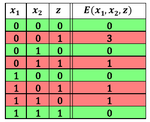
We can see that the energy is minimized on exactly the desired feasible configurations. So we encode this energy function as a QUBO. We make the offset 0.0 because there is no constant energy offset.

qubo = dimod.BinaryQuadraticModel({'x1': 0., 'x2': 0., 'z': 3.},
                               {('x1', 'x2'): 1., ('x1', 'z'): 2., ('x2', 'z'): 2.},
                               0.0,
                               dimod.BINARY)

We know from the table that our ground energy is 0, but we can calculate it using the qubo to check that this is true for the feasible configuration (0, 1, 0).

ground_energy = qubo.energy({'x1': 0, 'x2': 1, 'z': 0})

The last value that we need is the classical gap. This is the difference in energy between the lowest infeasible state and the ground state.

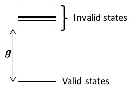
With all of the pieces, we can now build the penalty model.

classical_gap = 1
p_model = pm.PenaltyModel.from_specification(spec, qubo, classical_gap, ground_energy)

Installation

To install the core package:

pip install penaltymodel

License

Released under the Apache License 2.0

Contributing

Ocean's contributing guide has guidelines for contributing to Ocean packages.