Advanced Lane Finding

Lane Line Detection

---

The goals / steps of this project are the following:

• Compute the camera calibration matrix and distortion coefficients given a set of chessboard images.
• Apply a distortion correction to raw images.
• Use color transforms, gradients, etc., to create a thresholded binary image.
• Apply a perspective transform to rectify binary image ("birds-eye view").
• Detect lane pixels and fit to find the lane boundary.
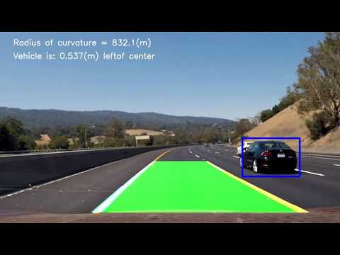
• Determine the curvature of the lane and vehicle position with respect to center.
• Warp the detected lane boundaries back onto the original image.
• Output visual display of the lane boundaries and numerical estimation of lane curvature and vehicle position.

Important files:

• LaneFinder.py
• LaneLinderFinder.py
• lanelines.py
• settings.py
• helpers.py
• Perspective transform.ipynb
• Camera_calibration.ipynb

We will break Lane Detection down into three stages:

Stage 1: Camera Distortion

• Our video stream was captured using a monocular camera. As such, we must correct the distortion that may occur. To do this, I used openCV's drawChessboardCoenrs and findChessboardCorners functions. I then created two lists, object_points and image_points. Object points describe's where each pixel in the image exists in a real world representation (X, Y, Z). Where image_points describe where each of those pixels are in the 2D .png image. We then compute the transformation matrix mtx and the distortion coefficient matrix dist, save them to a pickle file, because later on in stage 3 we will recall and use them in cv2.undistort().
• Code for this stage can be seen in Camera Calibration.ipynb
• You can see the original and undistorted images below
• 

Stage 2: Perspective Transformation (inside Perspective Transform.ipynb):

• Our goal in this stage is to find source and destination points that we can use to warp our perspective to obtain an aerial view of the road.

• This will allow us to calculate the distance in meters per pixel between the lane lines

• It is also easier to work with the warped image inside the laneLine's objects, because we are dealing with straight vertical lines instead of angles lines.

• (it's easier to see if our predicted lines are well drawn compared to the given lanes).

• Steps in this stage

• Read in the image

• Undistort the image (using the transformation matrix and distortion coefficients from Camera Calibration.ipynb

• Convert the image to HLS

• Apply canny edge detection on the Lightness layer of the HLS image. (This gives us a better representation of the lane lines).

• Apply the Hough Transform to obtain coordinates for lines that are considered to be straight

Finding the vanishing point:

The vanishing point in an image is the point where it looks like the picture can go on forever. If you recall photos of a sunset of a horizon where they appear to extend forever, that's the point we are looking for.

• a vanishing point is a point in the image plane where the projections of a set of parallel lines in space intersect.

• After we applied the Hough Transform we get coordinate sets inside a list

• The vanishing point is the the intersection of all the lines built from the coordinates inside that list

• It is the point with minimal squared distance from the lines in the hough list

• The total squared distance

• (1)

• where: I is the cost function, ni is the line normal to the hough lines and pi are the points on the hough lines

• Then we minimize I w.r.t vp.

• (2)

Finding source points:

To find the source points using the vanishing point vp, we had to be clever.

• So we have the vanishing point, which we can consider to be in the middle of our image. We want to locate a trapezoid that surrounds our lane lines.
• We first declare two points p1 and p2 which are evenly offset from the vanishing point, and are closer to our vehicle.
• Next, we want to find an additional two points p3 and p4 that exist on the line that connects p1 and vp, and p2 and vp.
• After that we will have the four points for our trapezoid (p1, p2, p3, p4), p1 and p4 live on the same line as do p2 and p3.
• We apply the equation (y2 - y1) = m (x2 - x1) and y = mx + b, and solve for x. (That is why we are using the inverse slope). This can be seen in find_pt_inline
• p1, p2, p3, and p4 form a trapezoid that will be our perspective transform region. our source points are [p1, p2, p3, p4].
• The source points define the section of the image we will use for our warping transformation
• The destination points are the where the source points will ultimately end up after we apply our warp. (pixels will be mapped from source points to destination points)
• 
• Here you can see the vanishing point (blue triangle)
• 
• Here you can see the Trapezoid mask we will be using for our perspective transform. The source points are marked with the + and ^ dots.

Finding the distance

• A lot of the methods applied here were suggested by ajsmilutin in this repository.
• We use moments in order to find the distance between two lane lines in our warped images.
• Lane lines are ~12 feet apart in the real world. We can use this info to find out how many pixels in our image equals 1 meter.
• We find the area between the lane lines using the zeroth moment, then we divide the first moment by the zeroth moment to get a centroid, (the center point) for both the right and left lane lines in the x-dimension.
• Now we find the minimum distance between the two centroids and define that to be our lane width. Then convert the lane width from feet to meters and now we have our pixels per meter in x. In our warped image there is no depth, it is planar. Therefore the Z in our homography matrix is 0. With that information, now all we have to do is determine the y-component from the x-component. We do this by scaling the x-dimension slot in the homography matrix by the y-dimension slot. Then we multiply that scaled value by our x_pixels_per_meter to obtain the y_pixels_per_meter.
• x_pixel_per_meter: 53.511326971489076
• y_pixel_per_meter: 37.0398121547
• 
• You can see the centroids as the marked points in this image
• Then we save everything to a pickle file and move on to our lane line identification stage.
• Code for this stage can be seen inside Perspective_Transform.ipynb

Stage 3: Lane Line Identification (inside LaneFinder.py and LaneLineFinder.py)

Step 1: Lane detection (LaneFinder.py)

Preprocessing:

• First we undistort the image
• Then we warp the image into an aerial view
• 

Filtering: (in LaneFinder.py lines 114 to 143)

• We first create two copies of our warped image, an hls and a lab colorspace copy.
• apply a median blur to both copies

Detect yellow lane:

• Restrict hue values > 30 because lines should typically be a similar color angle

• Restrict saturation values < 50 because it is just noise at this point

• Cutoff lightness values > 190

• AND the hls filter with the b layer in lab, for which values > 127.5 correspond to yellow

• Everything up to this point that we have detected is the nature (trees to the left and right of the lane)

• Create a mask that is everything EXCEPT this nature piece (NOT)

• AND the mask with lightness values < 245

• Perform morphological operations: Opening followed by Dilation. Which is considerd Tophat

• Kernel sizes were selected manually through trial and error. A larger kernel rules out more noise, and a smaller kernel is designed to pick up small disturbances.

• Tophat the lab, hls, and the yellow filter. Tophat reduces noise from tiny pixels. Tophat = opening + dilation. Read about it here

• See the filters here:

• This is what the hls luminance filter picked up:

• 

• Here is the hls saturation filter

• 

• Here is the region of interest filter (after we NOT the nature part)

• 

• Then we perform adaptive thresholding (LaneFinder.py lines 160-162)

• Then we combine this mask with the roi_mask to create a difference mask (shown below)

• 

• Then we perform erosion on the difference mask to obtain the total mask.

• I tried using 5x5 kernels at first for this erosion step. Ellipses were the best kernel shape because they will erode isolated pixels, but when the kernel size was (5, 5) it was too large and it started to erode the pixels that correspond to dashes inside the lane lines. So (3, 3) was the best option, even though occasionally it may remove pixels in between the lane lines.

• 

• Now we pass this binary mask into our LaneLineFinder instance.

Step 2: Line detection (LaneLineFinder.py)

• Input:

• 

• The LaneLineFinder finds one lane line, either left or right given a warped image (aerial view)

pt1: LaneLineFinder get_initial_coefficients (lines 123 to 188)

• Take the bottom vertical half of the image and compute the vertical sum of the pixel values (histogram)
• Find the max index, and use that as a starting point
• Then search for small window boxes from the bottom up to find the max pixel density (that is where the lane lines are)
• 
• Save the good centroids to a list
• Calculate the coefficients for the equation f(x) = ay^2 + by + c. You can see this line 188 as the result of np.polyfit

pt2: For the next frame, use get_next_coefficients (lines 71-86)

• Since we know where the lane lines were from the first frame, we don't have to start our search from scratch.
• Scan around the previous coefficients for the next lane line marking within a reasonable margin (line 77)
• We look within a margin for the next point, instead of scanning the entire image from scratch again
• If there is a large deviation from the average, then our line is not good, and we set our found property to false, then in our LaneFinder we will use the previous good line instead of this line
• You can see this feature in the video stream. When the lane line starts to drive off and deviate from the previous line it resets back to the previous good line
• Now we have the coefficients

pt3: Use get_line_pts (line 101 - 104)

• Here we pass in the coefficients and receive our X and Y values to plot.

pt4: Use draw_lines (line 116-131)

• Here we take in the x and y coordinates as fitx and plot_y respectively
• Then we calculate our lane points and fill a window with cv2.fillPoly. This gives us extra padding on the left and right of the line so it looks thick
• Then we pass our lane points into draw_pw (lines 106 - 114) which draws each segment inside a for loop
• Then we return the drawn lines to LaneFinder
• If the line wasn't detected we simply use the previous lane line.

pt5: Calculate curvature

• inside get_curvature line (190 - 204) we calculate the curvature following this procedure
• We use the x_pixels_per meter and y_pixels_per_meter that we found in our perspective transform notebook (stage 2)

last part: Receive lines in LaneFinder

• Then we receive the lines for the left and right lane line as LaneFinder.left_line and LaneFinder.right_line respectively.
• Then we use cv2.add_weighted with the warped image and the combination of both the lane lines.
• Then we unwarp the image and return it
• I calculated the center place using the last fit coordinates of the left and right lines
• I used the left fit coordinate and the right fit coordinates to determine the accurate indices to draw the middle lane. You can see this inside laneFinder lines (121 - 141)
• 

Video of result

Reflection

• I attempted to structure my basic outline similar to how ajsmilutin did in this repository. However my implementation details and methods are far different. I experimented with many different kernels, and it turns out, the ones he used in his process are the best. I tried to prove him wrong and use (29, 29)'s for the first erosion, but it ended up not working properly.
• In fact. I used a lot of what he did, and it took me a LONG time to wrap my head around how it works. The OOP structure he uses in his implementation was new to me, because I don't have that much experience with OOP programming in python, so I learned a lot by trying to reproduce what he did, except I did it in a very different way. I used the adaptive thresholding technique instead of doing sobelx, sobely, and magnitude gradients because it proves to be far better in performance on the challenge video. Even though I couldn't get the challenge video to work well for my implementation. Credit where credit is due, I learned a TON about filtering from ajsmulitin.
• I should have created a reset option, so that if the detected line deviates too far from the average we will do a complete reset and then look for the next line as if it was the first line. This would help solve the challenge video.
• I still need to create an averaging function so that the drawn lines are drawn from the coefficients of the previous 5 frames for smoothing.
• I also received the idea for using the histogram from Udacity's starter code.
• Originally I tried using a convolutional window, but it proved to not work as well. I was using a rectangular window for a very long time, and it was receiving outputs that did not correspond to the index of my max argument. Later on I discovered that I should be using a gaussian filter, so that the peak will be clear.
• I would not have been able to figure out how to use moments to find centroids with ajsmulitins code. It was hard for me to disect his code and see exactly what it was doing. Not an easy task.
• Special thanks to Kyle Stewart-Frantz who helped me think about how to find the deviations when I was completely stuck
• Originally I was working with jupyter notebooks, and then I got pycharm and my life changed when I figured out how to use the debugger. Completely necessary!!
• I used a pandas dataframe to test individual image sequences without having to process the entire video.I converted the video into a csv and img folder. The code for this can be seen in VideoAcquisition.ipynb

Vehicle Detection

Important files

• model.py (builds SVM classifier and trains on training data)
• Processor.py (overlaying processor that runs the pipeline on a video stream input)
• settings.py (settings for tuned parameters)
• Car_Detector.py (contains Car_Detector class that applies the model to detect cars and draws rectangular boxes on images)
• helpers.py (contains helper functions for feature extraction and sliding window implementation)

Training data:

• Our training dataset consists of 17760 images. 8792 non-vehicles and 8968 vehicles. We split our training and validation sets with 80% 20% respectively. So our training dataset was ~14208 images. The data looks like this

Process:

1) Training data (model.py)

• Grab the training data and extract image paths and store them in the model class
• Train a linear Support Vector Machine (lines 54 - 57)
• Split the training data using train_test_split. Keep in mind that we are using training data as validation data, so there is some overfitting there. On a time series analysis it would be more robust to check a time-range and split validation data so that it has distinct times from the training data
• Normalize the training data using mean - std normalization, using scikit's StandardScaler (line 49)
• Set the LinearSVC's C parameter to 0.01 so that it's predictions will be less attached to the dataset and able to generalize better
• Train the model on the data
• Save the LinearSVC (Linear Support Vector Machine) to a pickle file as well as other parameters and move to step 2 (line 79)

2) Car detection (helpers.py)

In Car_helpers.find_cars (helpers.py) implemented in get_detections() inside Car_Detector.py

Sliding Window Implementation

Instead of creating random sliding windows, extract features from an entire region of the image, and then use those cells to determine if there is a vehicle present.

• Extract out a section of the image (height from ystart to ystop as defined by the function caller in Car_Detector.py) and all width.
• Extract the HOG features for the entire section of the image
• Here is what HOG features gives us

• 
• Above: You can see the region we are using for our sub image between the light and dark blue lines
• Scale the extracted section by a scale parameter (line 168)
• Extract each channel from the scaled image
• Calculate the number of blocks in x and y
• Create multiple search windows with different scales and different regions (I used 3)
• Create a step size (cells_per_window / step_size) = % overlap
• Discover how many vertical and horizontal steps you will have
• Calculate HOG features for each channel lines
• Consider the scaled image to be in position space, not image space. We treat sections of the image as a grid in terms of whole integer values instead of in pixel values. See image below on how to grid looks

• We will move from grid space back into image space later on don't worry
• For now, consider xpos and ypos to be grid positions (from left to right)
• Iterate through the grid (in y then x) lines
• Grab a subsample of the hog features corresponding to the current cell
• stack the features (line 203)
• go from grid space to pixel space now xleft and ytop are in image space
• extract the image patch (as defined by the boundaries of xleft and ytop and the window size)
• get the spatial and histogram features using spatial_features and hist_features which are defined in helpers.py
• Normalize the features using X_scaler from model.py
• Stack the features
• Compute the prediction from the Support Vector Machine and the confidence
• If the prediction is 1 and the decision function confidence is > 0.6 then we have detected a car
• Rescale xbox_left and ytop_draw to go from our current image space (which is scaled) to real image space by multiplying it by the scaling factor scale
• Use the drawing window dimensions to build (x1, y1, x2, y2) detection coordinates which will help us build a heatmap for the detected cars location
• Add those detections to our detections list

In Car_Finder.get_centroid_rectangles

• Take in the output from Car_Finder.find_cars (which are the detection coordinates above)

• Take in the detection coordinates and update the heatmap by adding 5 to each value within the heatmap's bounding box

• 

• Above, as you can see we have more than one bounding box. Therefore we need to apply a heatmap in order to determine an accurate region for the vehicle and only draw one box

• 

• As you can see, sometimes we get detections that are false positives, in order to remove these false positives we apply a thresholding function

• Remove the values where the heatmap's values are < threshold. So it takes ~4 heat maps to pass through the thresholder

• Before we threshold, we take an average of the last 10 heat maps if 10 heat maps have been saved, then we insert this map into our thresholder

• Averaging allows us to rule out bad values and creates a smoother transition between frames

• Then we find the contours for the binary image, (which are basically the large shapes created from the heatmap)

• Then we create bounding boxes from these contours

• 

• Above you can see that we have some false positives in the opposing lane, therefore we will rule out any boxes that occur at width < 50 because this area corresponds to the opposing highway. We do this on line 91

• Grab the coordinates of the bounding box and append them to centroid_rectangles which we will pass to our draw_centroids helper function

Draw Centroids (in helpers.py)

• Get the centroid coordinates and the original image and draw a rectangle with the coordinates given
• Return this image.
• Note: I got the idea to find the contours from Kyle Stewart-Frantz

Helper functions (in helpers.py)

• Extract_features (lines 61 - 112). This function takes in list of image paths, reads the images, then extracts the spatial, histogram, and hog features of those images and saves them. This occurs in our preprocessing pipeline when we are training the model. Our SVM does not extract features itself, so we have to extract them from images, similar to how a multi-layer perceptron works, in contrast with how CNN's work.
• We extract features using three helper functions:
• bin_spatial : This function resizes our image to a desired size and then flattens it, giving us the pixel values in a flattened row vector
• color_hist: This function computes the histogram for each color channel and then concatenates them together
• get_hog_features: This function computes the histogram of oriented gradient and returns a 1-D array of the HOG features
• Then inside Extract_features we grab all of these features for each image and then add them to our features list. So features contains the features for the entire data set where a file_feature contains the features for one image THE END

Details (Parameter selection) (tuning params.ods)

Color Space:

• 
• Above: I tried these different parameters and tested the SVM's predictions on a single image. I chose the YCrCb ALL channel color space because it gave me the best accuracy at training time
• 
• Above: Result of training using YCrCb color space
• This gives us the best result with an accuracy of 99.5. Don't be fooled by the 1.0 in the grid of parameter tests, that was only sampled for one image
• 
• Above: Result of training using L channel in LUV color space
• 
• Above: Result of training using V channel in LUV color space

Orientations:

• I chose to use 9 orientations

Performance Optimizations:

• I stored all my image paths in a pandas dataframe. I processed each image and viewed the results to see how well my pipeline works. When using the summing method, I started out with a threshold of 0.6 * 10 ~ 60. I later tuned this threshold to be 0.58 * 10 = 58. If I used 56 I would start drawing boxes in the middle of the road.
• I did not create a new image to draw on each time, I simply drew on the input image. I didn't want to process more things.

Video of result

Final Result Image:

Reflection:

I tried a lot of different methods to get the most accurate pipeline. In theory, saving the state of the heatmap for subsequent images should work if you cool the regions where there are not current detections. This approach seems to work fairly well as you can see in the Video for heatmap cooling above. However, it involves storing more information because you have to save the state of the current heatmap to memory and it increases computation time. I like the idea of it, although determining the thresholds for it was rather difficult and involved a fair amount of evaluation.

The heatmap summming approach allows me to work with whole number thresholds instead of decimal thresholds (which are used in the averaging approach). Other than that it performs relatively the same as the averaging approach. I scaled the threshold value based on the number of heatmaps that are stored in the heatmaps queue.

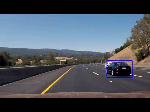
As I pass through the lightly colored road I lose a detection on the white vehicle. This is simply due to the model parameters and the prediction constraints. At this point I do not have an accurate prediction, so no bounding box is drawn. The model is only as good as the data.

At one point in the video the bounding box splits into two bounding boxes when it should be one bounding box. This happened because cv2.findContours found two contours due to the upper and lower section of the bounding boxes.

(Above) as you can see in this case the [cv2.findContours](http://docs.opencv.org/trunk/d4/d73/tutorial_py_contours_begin.html) function inside get_centroid_rectangles detects two different contours, and that's why two bounding boxes were drawn.

Twitter: @jonathancmitch

Linkedin: https://www.linkedin.com/in/jonathancmitchell

Github: github.com/jonathancmitchell

Medium: https://medium.com/@jmitchell1991

Tools used

• Numpy
• OpenCV3
• Python
• Pandas
• Matplotlib
• SciKit-Learn