In this tutorial we'll go over how to use QIIME 2 to analyze metabarcoding data. We'll start with an introduction about how metabarcoding (aka amplicon) data is produced and with a refresher for working in the BASH command-line environment.
DNA taxonomy in a broad sense, means any form of analysis that uses variation in DNA sequence data to inform species delimitation.
Barcoding - identification (taxonomically/phylogenetically) of an organism by a short section of DNA/RNA, usually through PCR amplification with conserved DNA/RNA primers.
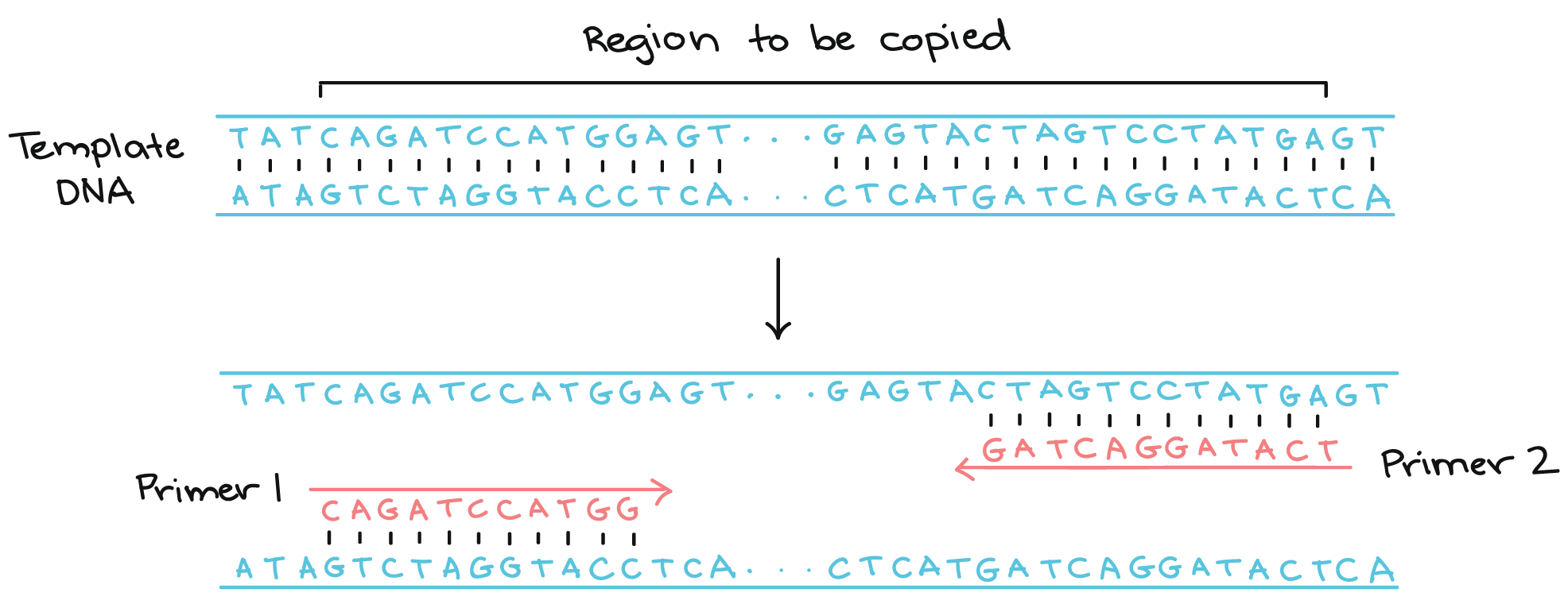
Polymerase chain reaction (PCR) - an amplification technique for cloning the specific or targeted parts of a DNA sequence to generate thousands to millions of copies of DNA of interest.
Metabarcoding - barcoding of DNA/RNA or eDNA/eRNA in a manner that allows for identification of many taxa within the same sample. Also known as "amplicon" sequencing, or "marker gene sequencing".
eDNA - environmental DNA.
Metagenomics - en mass sequencing of a community of organisms using whole-genome shotgun sequencing
| Collect Sample | Extract DNA |
|---|---|
 |
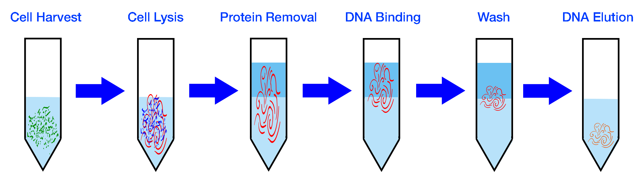 |
| PCR Amplification | Repeat for x Cycles |
|---|---|
 |
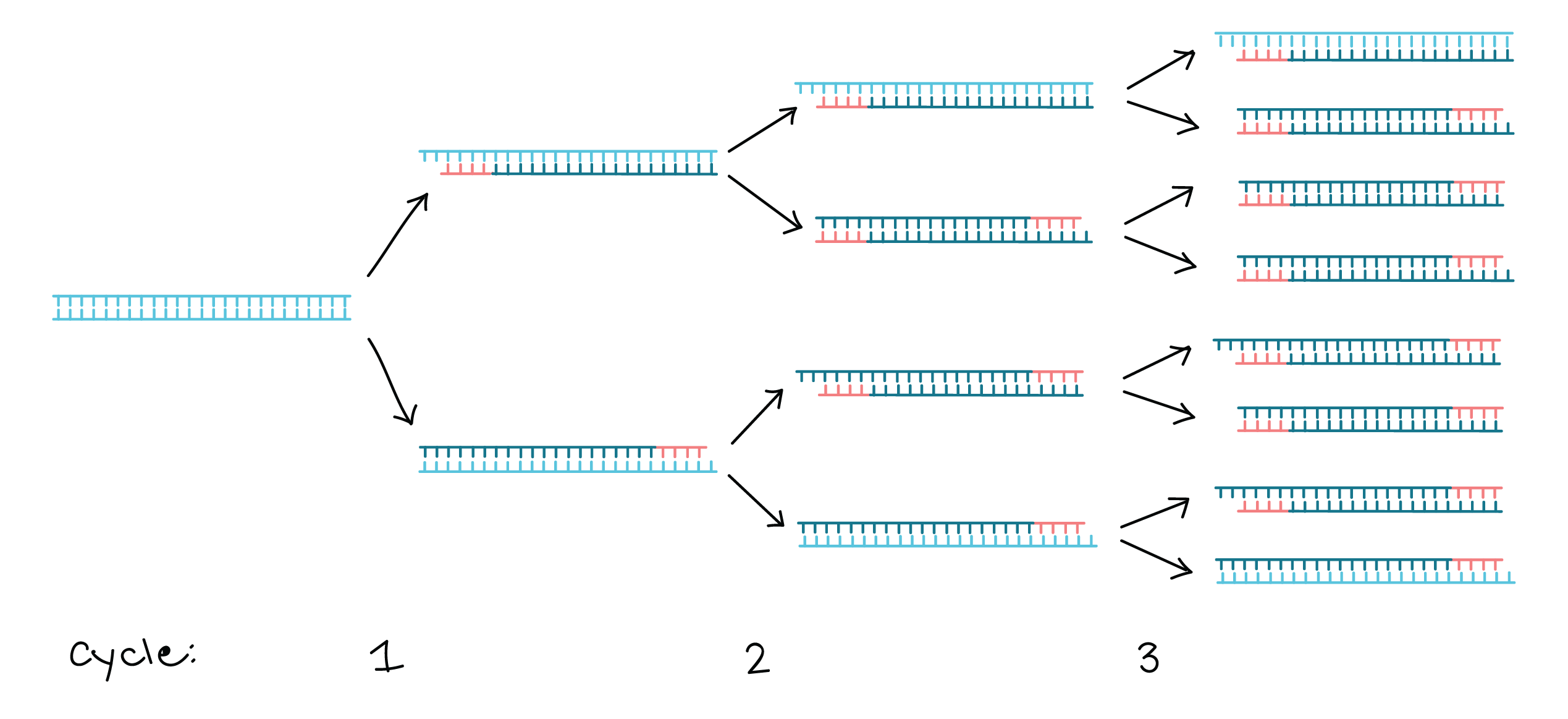 |
| Prepare Library | Sequence DNA |
|---|---|
 |
 |
image references:

Selecing a locus for barcoding
-
The targeted region should have little intraspecific variation (< 2% sequence identity) and enough interspecific variation (>2% sequence identity) to distinguish different species.
-
It should be phylogenetically informative to allow the placement of newly barcoded organisms to accurate lineages.
-
The primer binding sites should be highly conserved and specific, so DNA amplification is reliable across all taxa in question. This is especially important for en mass community analyses (metabarcoding) and will make the development of universal primers more efficient and help alleviate potential PCR bias.
-
For studies utilizing HTS the target region must be small enough to be recovered on one or two sequencing reads when using paired-end information (<600 bps). Shorter sequences are also preferred for recovering barcoding sequences from preserved or degraded samples.
-
Reference sequence databases with taxonomic information exists for the region in question.
| Target-Organisms | Gene | Region | Location/Name | Length (bp) | Forward-primer | Reverse-primer | F_length | R_length | Reference |
|---|---|---|---|---|---|---|---|---|---|
| Prokaryotes | 16S | V4 | 515F-806R | ~390 | GTGYCAGCMGCCGCGGTAA | GGACTACNVGGGTWTCTAAT | 19 | 20 | Walters et al. 2016 |
| Prokaryotes | 16S | V4-V5 | 515-926R | ~510 | GTGYCAGCMGCCGCGGTAA | CCGYCAATTYMTTTRAGTTT | 19 | 20 | Stoek et al. 2010 |
| Microbial Eukaryotes | 18S | V9 | 1391F-1510R | ~210 - 310 | GTACACACCGCCCGTC | TGATCCTTCTGCAGGTTCACCTAC | 16 | 24 | Amaral-Zettler et al. 2009 |
| Fungal and micro euks | ITS | ITS1-ITS2 | ITS1F-ITS2 | ~250 - 600 | CTTGGTCATTTAGAGGAAGTAA | GCTGCGTTCTTCATCGATGC | 22 | 20 | White et al., 1990 |
| Fish | 12S | V5 | MiFish | ~163 - 185 | GTCGGTAAAACTCGTGCCAGC | CATAGTGGGGTATCTAATCCCAGTTTG | 21 | 27 | Miya et al, 2015 |
For each program that we run in this tutorial I have provided a link to the manual. These manuals provide a thorough explanation of what exactly we are doing. Before running the workflow on your own data you should read the manual/publication for the program.
Throughout this tutorial the commands you will type are formatted into the gray text boxes (don't do it when learning but they can be faithfully copied and pasted). The '#' symbol indicates a comment, BASH knows to ignore these lines.
This tutorial assumes a general understanding of the BASH environment. You should be familiar with moving around the directories and understand how to manipulate files.
Remember to tab complete! There is a reason the tab is my favorite key. It prevents spelling errors and allows you to work much faster. Remember if a filename isn't auto-completing you can hit tab twice to see your files while you continue typing your command. If a file doesn't auto-complete it means you either have a spelling mistake, are in a different directory than you originally thought, or that it doesn't exist.
See the BASH tutorials to get started.
This is important and ensures that all the programs we use are updated and in working order. You'll need to do this every time you login to the server and need general bioinformatic tools.
conda activate genomics

conda info --envs
# setup working directory
mkdir ~/bash-practice
cd ~/bash-practice

# copy example reads
cp -r /home/share/examples/example-reads/ ./
Link explaining the 'Read Name Format': SampleName_Barcode_LaneNumber_001.fastq.gz
Note the file extension - fastq.gz. Since these files are usually pretty big it is standard to receive them compressed. To view these files ourselves (which you normally wouldn't do) you either have to decompress the data with gunzip or by using variations of the typical commands. Instead of 'cat' we use 'zcat', instead of grep we can use 'zgrep'. Or just use less which allows you to stream a zipped file for viewing.
less -S example-reads/*_R1_*Each sequencing read entry is four lines long..
- Line 1. Always begins with an '@' symbol and denotes the header. This is unique to each sequence and has info about the sequencing run.

- Line 2. The actual sequencing read for your organism, a 250 bp string of As, Ts, Cs, and Gs.

- Line 3. Begins with a '+' symbol, this is the header for the read quality. Usually the same as the first line header.

- Line 4. Next are ascii symbols representing the quality score (see table below) for each base in your sequence. This denotes how confident we are in the base call for each respective nucleotide. This line is the same length as the sequencing line since we have a quality score for each and every base of the sequence.


- Count The Number of Raw Reads
I always start by counting the number of reads I have for each sample. This is done to quickly assess whether we have enough data to assemble a meaningful genome. Usually these file contains millions of reads, good thing BASH is great for parsing large files! Note that the forward and reverse reads will have the same number of entries so you only need to count one.
# using grep. Note that I don't count just '@', this is because that symbol may appear in the quality lines.
zgrep -c '^@' Sample*/*R1*
# counting the lines and dividing by 4. Remember each read entry is exactly four lines long. These numbers should match.
zcat Sample*/*_R1_* | wc -l- Whats our total bp of data? This is what we call our sequencing throughput. We multiple the number of reads by the read length (ours is 250) and by 2 because it is paired-end data.
(Read length x 2(paired-end) x Number of reads)
# we can do this calculation from the terminal with echo and bc (bc is the terminal calculator)
echo "Number_of_reads * 250 * 2" | bc
program: FASTQC
manual: https://www.bioinformatics.babraham.ac.uk/projects/fastqc/
- Run Fastqc
FastQC is a program to summarize read qualities and base composition. Since we have millions of reads there is no practical way to do this by hand. We call the program to parse through the fastq files and do the hard work for us. The input to the program is one or more fastq file(s) and the output is an html file with several figures. The link above describes what each of the output figures are describing. I mainly focus on the first graph which visualizes our average read qualities and the last figure which shows the adapter content. Note that this program does not do anything to your data, as with the majority of the assessment tools, it merely reads it.
# make a directory to store the output
mkdir fastqc_raw-reads
# run the program
fastqc example-reads*/*_R1_* example-reads*/*_R2_* -o fastqc_raw-reads
ls fastqc_raw-reads
# the resulting folder should contain a zipped archive and an html file, we can ignore the zipped archive which is redundant.- Transfer resulting HTML files to computer using filezilla or with the command line on OSX/Linux.
On filezilla you will need to enter the same server information when you login form the terminal. Be sure to use port 22.
# to get the absolute path to a file you can use the ‘readlink’ command.
readlink -f fastqc_raw-reads/*.html
# copy those paths, we will use them for the file transfer
# In a fresh terminal on OSX, Linux, or BASH for windows
scp USERNAME@ron.sr.unh.edu:/home/GROUP/USERNAME/mdibl-t3-2019-WGS/fastqc_raw-reads/*.html /path/to/put/files- Transfer resulting HTML files to computer using filezilla or with the command line on OSX/Linux.
On filezilla you will need to enter the same server information when you login form the terminal. Be sure to use port 22.
# to get the absolute path to a file you can use the ‘readlink’ command.
readlink -f fastqc_raw-reads/*.html
# copy those paths, we will use them for the file transfer
# In a fresh terminal on OSX, Linux, or BASH for windows
scp USERNAME@ron.sr.unh.edu:/home/GROUP/USERNAME/bash-practice/fastqc_raw-reads/*.html /path/to/put/files

"QIIME 2™ is a next-generation microbiome bioinformatics platform that is extensible, free, open source, and community developed."
These data are from set of mouse fecal samples provided by Jason Bubier from The Jackson Laboratory. The samples were run targeting the V1-V3 region of the 16S gene using the 27F - 534R primer pair on an Illumnina MiSeq on a paired end 300 bp run.
27F [20 bp]
 5'AGM GTT YGA TYM YGG CTC AG
534R [17 bp]
 5'ATT ACC GCG GCT GCT GG
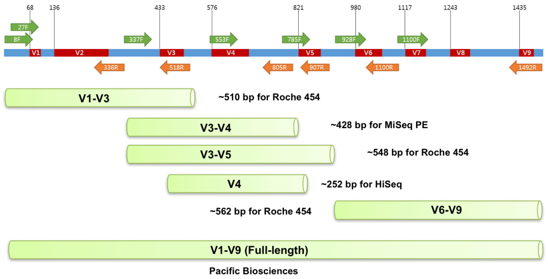
image source - https://help.ezbiocloud.net/16s-rrna-and-16s-rrna-gene/
For Metadata we have the sex, strain, and age (# days). Our goal is to examine the correlation of the fecal microbiome we observe with these metadata. We will primarily use the Qiime 2 bioinformatics platform. Qiime 2 is free and open source and available from Linux and OSX. We will use the Qiime2 command line interface, there is also the "Artifact" python API which can be more powerful.
mkdir hcgs-qiime2-workshop
cd hcgs-qiime2-workshop
cp -r /home/share/examples/cocaine_mouse/* .
ls

# mdat.tsv

less -S mdat.tsv
#SampleID       Sex     Treatment       Strain  Date    PrePost Dataset HaveBred        PerformedPCR    Description     pptreatment     Testing
#q2:types       categorical     categorical     categorical     numeric categorical     categorical     categorical     categorical             categorical     categorical
JBCDJ00OLJ1STT0B00000191821C7M7FGT1904904       F       Sham    CC004   0       Pre     Dataset1                Jax     19182_1 PreSham Train
JBCDJ00OLK1STT0B00000191671C7M7FGT1904905       F       Coc     CC041   0       Pre     Dataset1                Jax     19167_1 PreCoc  Train
JBCDJ00OLL1STT0B00000191771C7M7FGT1904906       M       Sham    CC004   0       Pre     Dataset1                Jax     19177_1 PreSham Test
JBCDJ00OLM1STT0B00000191861C7M7FGT1904907       M       Coc     CC004   0       Pre     Dataset1                Jax     19186_1 PreCoc  Test
JBCDJ00OLN1STT0B00000191791C7M7FGT1904908       F       Coc     CC004   0       Pre     Dataset1                Jax     19179_1 PreCoc  Train
JBCDJ00OLO1STT0B00000191691C7M7FGT1904909       F       Sham    CC041   0       Pre     Dataset1                Jax     19169_1 PreSham Test
JBCDJ00OLP1STT0B00000191731C7M7FGT1904910       M       Coc     CC041   0       Pre     Dataset1                Jax     19173_1 PreCoc  Test
JBCDJ00OLQ1STT0B00000191641C7M7FGT1904911       M       Coc     CC041   0       Pre     Dataset1                Jax     19164_1 PreCoc  Train
JBCDJ00OLR1STT0B00000191801C7M7FGT1904912       F       Sham    CC004   0       Pre     Dataset1                Jax     19180_1 PreSham Train
JBCDJ00OLS1STT0B00000191831C7M7FGT1904913       F       Coc     CC004   0       Pre     Dataset1                Jax     19183_1 PreCoc  Train
JBCDJ00OLT1STT0B00000191841C7M7FGT1904914       M       Sham    CC004   0       Pre     Dataset1                Jax     19184_1 PreSham Train
JBCDJ00OLU1STT0B00000191711C7M7FGT1904915       M       Coc     CC041   0       Pre     Dataset1                Jax     19171_1 PreCoc  Train
JBCDJ00OLV1STT0B00000191681C7M7FGT1904916       F       Sham    CC041   0       Pre     Dataset1                Jax     19168_1 PreSham Train
When we look at the metadata file we see the metadata that we will be able to use during our analysis
## Anatomy of a qiime command
qiime plugin action\
   --i-inputs  foo\       ## input arguments start with --i
   --p-parameters bar\    ## paramaters start with --p
   --m-metadata mdat\     ## metadata options start with --m
   --o-outputs out        ## and output starts with --o
Qiime works on two types of files, Qiime Zipped Archives (.qza) and Qiime Zipped Visualizations (.qzv). Both are simply renamed .zip archives that hold the appropriate qiime data in a structured format. This includes a "provenance" for that object which tracks the history of commands that led to it. The qza files contain data, while the qzv files contain visualizations displaying some data. We'll look at a quality summary of our reads to help decide how to trim and truncate them.
qiime tools import\
   --type 'SampleData[PairedEndSequencesWithQuality]'\
   --input-path manifest.csv\
   --output-path demux\
   --input-format PairedEndFastqManifestPhred33
## the correct extension is automatically added for the output by qiime.Now we want to look at the quality profile of our reads. Our goal is to determine how much we should truncate the reads before the paired end reads are joined. This will depend on the length of our amplicon, and the quality of the reads.
qiime demux summarize\
   --i-data demux.qza\
   --o-visualization demux
When looking we want to answer these questions:
How much total sequence do we need to preserve an sufficient overlap to merge the paired end reads?
How much poor quality sequence can we truncate before trying to merge?
In this case we know our amplicons are about 390 bp long, and we want to preserve approximately 50 bp combined overlap. So our target is to retain ~450 bp of total sequence from the two reads. 450 bp/2 = 225 bp but looking at the demux.qzv, the forward reads seem to be higher quality than the reverse, so let's retain more of the forward and less of the reverse.
We're now ready to denoise our data. Through qiime we will be using the program DADA2, the goal is to take our imperfectly sequenced reads, and recover the "real" sequence composition of the sample that went into the sequencer. DADA2 does this by learning the error rates for each transition between bases at each quality score. It then assumes that all of the sequences are errors off the same original sequence. Then using the error rates it calculates the likelihood of each sequence arising. Sequences with a likelihood falling below a threshold are split off into their own groups and the algorithm is iteratively applied. Because of the error model we should only run samples which were sequenced together through dada2 together, as different runs may have different error profiles. We can merge multiple runs together after dada2. During this process dada2 also merges paired end reads, and checks for chimeric sequences.
qiime dada2 denoise-paired\
   --i-demultiplexed-seqs demux.qza\
   --p-trim-left-f 20 --p-trim-left-r 17\
   --p-trunc-len-f 295 --p-trunc-len-r 275\
   --p-n-threads 18\
   --o-denoising-stats dns\
   --o-table table\
   --o-representative-sequences rep-seqs
Now lets visualize the results of Dada2.
## Metadata on denoising
qiime metadata tabulate\
   --m-input-file dns.qza\
   --o-visualization dns
## Unique sequences accross all samples
qiime feature-table tabulate-seqs\
   --i-data rep-seqs.qza\
   --o-visualization rep-seqs
## Table of per-sample sequence counts
qiime feature-table summarize\
   --i-table table.qza\
   --m-sample-metadata-file mdat.tsv\
   --o-visualization table
Looking at dns.qzv first we can see how many sequences passed muster for each sample at each step performed by dada2. Here we are seeing great final sequence counts, and most of the sequences being filtered in the initial quality filtering stage. Relatively few are failing to merge, which suggests we did a good job selecting our truncation lengths.
In the table.qzv we can see some stats on our samples. We have millions of counts spread across thousands of unique sequences and tens of samples. We'll come back to the table.qzv file when we want to select our rarefaction depth.
In the rep-seqs.qzv we can see the sequences and the distribution of sequence lengths. Each sequence is a link to a web-blast against the ncbi nucleotide database. The majority of the sequences we observe are in our expected length range. Later on we can use this to blast specific sequences we are interested in against the whole nucleotide database.
qiime tools extract --input-path table.qza --output-path extracted-table biom convert -i extracted-table/*/data/feature-table.biom -o feature-table.tsv --to-tsv qiime tools extract --input-path rep-seqs.qza --output-path extracted-seqs
VSEARCH uses a fast heuristic based on words shared by the query and target sequences in order to quickly identify similar sequence
The main qiime2 tutorials utilizes a pre-trained Naive Bayes classifier (machine learning) and the q2-feature-classifier plugin. Here we will utilize Vsearch which works well out-of-the-box for most datasets. The output is similiar to BLAST.
qiime feature-classifier classify-consensus-vsearch\
   --i-query rep-seqs.qza\
   --i-reference-reads /home/share/databases/SILVA_databases/silva-138-99-seqs.qza\
   --i-reference-taxonomy /home/share/databases/SILVA_databases/silva-138-99-tax.qza\
   --p-maxaccepts 5 --p-query-cov 0.4\
   --p-perc-identity 0.7\
   --o-classification taxonomy\
   --p-threads 72
qiime metadata tabulate\
--m-input-file taxonomy.qza\
--o-visualization taxonomy.qzv
qiime taxa barplot --i-table table.qza\
--i-taxonomy taxonomy.qza\
--o-visualization taxa-barplot\
--m-metadata-file mdat.tsvOur next step is to look at the diversity in the sequences of these samples. Here we will use the differences between the sequences in the sample, and metrics to quantify those differences to tell us about the diversity, richness and evenness of the sequence variants found in the samples. In doing so we will construct a de novo phylogenetic tree, which works much better if we first remove any spurious sequences that are not actually the target region of our 16S gene. To do that we will use our taxonomic assignments to filter out sequences that remained Unassigned, are assigned only as Bacteria or are Eukaryotes. We should look at what we are filtering out and try and find out what it is.
## exact match to filter out unassigned and Bacteria
## exact because bacteria is part of many other that we want to keep.
qiime taxa filter-table\
   --i-table table.qza\
   --i-taxonomy taxonomy.qza\
   --p-exclude "Unassigned,D_0__Bacteria"\
   --p-mode exact\
   --o-filtered-table bacteria-table

## Partial match to Eukaryota to filter out any Euks
qiime taxa filter-table\
   --i-table bacteria-table.qza\
   --i-taxonomy taxonomy.qza\
   --p-exclude "Eukaryota"\
   --o-filtered-table bacteria-table2

mv bacteria-table2.qza bacteria-table.qza

## Any additional sequences that we should exclude can be filtered on a "per feature basis"
## In this case we had some sequences that look like they were sequenced backwards!

qiime feature-table filter-features\
   --i-table bacteria-table.qza\
   --m-metadata-file exclude.tsv\
   --p-exclude-ids\
   --o-filtered-table bact-table.qza

## How much did we filter out?
qiime feature-table summarize\
   --i-table bacteria-table.qza\
   --m-sample-metadata-file mdat.tsv\
   --o-visualization bacteria-table

## Does it look very different?
qiime taxa barplot --i-table bacteria-table.qza\
   --i-taxonomy taxonomy.qza\
   --o-visualization bacteria-taxa-barplot\
   --m-metadata-file mdat.tsv

## Filter the sequences to reflect the new table.
qiime feature-table filter-seqs\
   --i-table bacteria-table.qza\
   --i-data rep-seqs.qza\
   --o-filtered-data bacteria-rep-seqs

qiime feature-table tabulate-seqs\
   --i-data bacteria-rep-seqs.qza\
   --o-visualization bacteria-rep-seqs
Now that we have only our target region we can create the de novo phylogenetic tree. We'll use the default qiime2 pipeline because it is quick and easy to run, while providing good results. This pipeline first performs a multi sequence alignment with mafft, this alignment would be significantly worse if we had not removed the non target sequences. It then masks highly variable parts of the sequence as they add noise to the tree. It then uses FastTree to create an unrooted phylogenetic tree which is then midpoint rooted.
qiime phylogeny align-to-tree-mafft-fasttree\
   --i-sequences bacteria-rep-seqs.qza\
   --o-alignment aligned-rep-seqs.qza\
   --o-masked-alignment masked-aligned-rep-seqs.qza\
   --o-tree unrooted-tree.qza\
   --o-rooted-tree rooted-tree.qza\
   --p-n-threads 18
Now we can look at the tree we created on iToL. And for reference here is the tree if we had not filtered it. We can see that the filtering upped the contrast between different groups.
Now we are ready to run some diversity analysis! We are going to start by running qiimes core phylogenetic pipeline, this will take into account the relationships between sequences, as represented by our phylogenetic tree. It will calculate a few key metrics for us, faiths-pd a measure of phylogenetic diversity, evenness, a measure of evenness and several beta statistics, like weighted and unweighted unifracs. To do these comparisons we need to make our samples comparable to each other. The way this is generally done is to rarefy the samples to the same sampling depth. We can use the bacteria-table.qzv we made earlier to inform this decision. We want to balance setting as high as possible of a rarefaction depth to preserve as many reads as possible, while setting it low enough to preserve as many samples as possible.
https://docs.qiime2.org/2022.2/plugins/available/diversity/alpha-rarefaction/?highlight=rarefaction
https://www.drive5.com/usearch/manual/rare.gif
qiime diversity alpha-rarefaction --i-table bacteria-table.qza --i-phylogeny rooted-tree.qza --p-max-depth 5000 --p-steps 100 --m-metadata-file mdat.tsv --o-visualization alpha-rarefaction.qzv
qiime diversity core-metrics-phylogenetic\
   --i-phylogeny rooted-tree.qza\
   --i-table bacteria-table.qza\
   --p-sampling-depth 16951\
   --m-metadata-file mdat.tsv\
   --output-dir core-metrics-results
From this initial step we can start by looking at some PCoA plots, we'll augment the PCoA with some of the most predictive features.
qiime feature-table relative-frequency\
   --i-table core-metrics-results/rarefied_table.qza\
   --o-relative-frequency-table core-metrics-results/relative_rarefied_table

qiime diversity pcoa-biplot\
   --i-features core-metrics-results/relative_rarefied_table.qza\
   --i-pcoa core-metrics-results/unweighted_unifrac_pcoa_results.qza\
   --o-biplot core-metrics-results/unweighted_unifrac_pcoa_biplot

qiime emperor biplot\
   --i-biplot core-metrics-results/unweighted_unifrac_pcoa_biplot.qza\
   --m-sample-metadata-file mdat.tsv\
   --o-visualization core-metrics-results/unweighted_unifrac_pcoa_biplot
We can see that the strains separate well, which implies that we should be able to find some separating distances in our data.
Lets start looking for those differences by looking at differences in diversity as a whole. For numeric metadata categories we can plot our favorite metrics with the value of that metadata.
qiime diversity alpha-correlation\
   --i-alpha-diversity core-metrics-results/faith_pd_vector.qza\
   --m-metadata-file mdat.tsv\
   --o-visualization core-metrics-results/faith-alpha-correlation
Then for the categorical metadata catagories we can plot some box and whisker plots.
qiime diversity alpha-group-significance\
   --i-alpha-diversity core-metrics-results/faith_pd_vector.qza\
   --m-metadata-file mdat.tsv\
--o-visualization core-metrics-results/faith-group-significanceNow lets combine the taxonomy with the diversity analysis to see if there are related groups of organisms that are differentially abundant groups within the samples. We'll start by combining our table and tree into a hierarchy and set of balances. Balances are the weighted log ratios of sets of features for samples. And we will be looking for significant differences in the balances between groups of samples.
qiime gneiss ilr-phylogenetic\
   --i-table bacteria-table.qza\
   --i-tree rooted-tree.qza\
   --o-balances balances --o-hierarchy hierarchy
To view the sets used in the balances we can plot out a heatmap of feature abundance which highlights the ratios.
qiime gneiss dendrogram-heatmap\
   --i-table bacteria-table.qza\
   --i-tree hierarchy.qza\
   --m-metadata-file mdat.tsv\
   --m-metadata-column Strain\
   --p-color-map seismic\
   --o-visualization heatmap.qzv
With this we can begin to look at specific balances to see their composition.
for ((i=0; i<10; i++)); do
  qiime gneiss balance-taxonomy\
     --i-table bacteria-table.qza\
     --i-tree hierarchy.qza\
     --i-taxonomy taxonomy.qza\
     --p-taxa-level 5\
     --p-balance-name y$i\
     --m-metadata-file mdat.tsv\
     --m-metadata-column Strain\
     --o-visualization y${i}_taxa_summary.qzv
done