This is a preliminary simulation study conducted in order to explain why bifactor models fit significantly better than higher order factor models. See https://osf.io/xp869/ for the official final study and documentation.
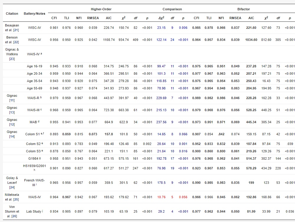
The aim was to test the suggestion by Kan et al (2020) that if a network model is the actual data generating mechanism, a bifactor model will likely outperform the higher order factor model in summarizing the data.
To this end we first simulate data according three models:
- A (second order) g model
- A bifactor model
- A network model extracted from the US standardization sample and refitted (confirmatory) on the German standardization sample correlation matrix.
Next, we fit all three models on all these data. This in order to show that the AIC and BIC would pick the true model, if the true model would be in the set of models considered.
Next, we show the results in case the network model would not be considered and the competition is between the higher order factor model and bifactor model. In that case the bifactor indeed beats the higher order factor model.
As, mentioned, the data concerned the WAIS-IV German validation sample data (correlation matrix). With thanks to Jens Lange for providing these data.
Let's clear our workspace first (run this line only if you really want that; you will lose everything you had in the workspace)
rm( list = ls() )
Load required packages and some helper functions
library( "psychonetrics" )
library( "dplyr" )
library( "devtools" )
source_url( 'https://raw.githubusercontent.com/KJKan/pame_I/main/R/helperfunctions.R' )
Our aim is to use a WAIS-IV network extracted previously (Kan et al., 2020) and to refit that network (confirmatory) in the German standardization sample. So let's load these matrices.
load( url ( "https://github.com/KJKan/pame_I/blob/main/data/WAIS_US.Rdata?raw=true" ) )
load( url ( "https://github.com/KJKan/pame_I/blob/main/data/WAIS_Germany.Rdata?raw=true" ) )
The sample sizes are:
n_US      <- 1800
n_Germany <- 1425
What subtests does the WAIS-IV include?
yvars <- colnames( WAIS_US )
These are:
- Block Design (BD)
- Similarities (SI)
- Digit Span (DS)
- Matrix Reasoning (MR or MA)
- Vocabulary (VC or VO)
- Arithmetic (AR)
- Symbol Search (SS)
- Visual Puzzles (VP)
- Information (IN)
- Coding (CO)
- Letter Number Sequencing (LN)
- Figure Weights (FW)
- Comprehension (CO)
- Cancellation (CA)
- Picture Completion (PC)
# Number of observed variables
ny        <- length( yvars )
15 in total.
# covariance matrix used in psychonetrics models
cov       <- ( n_Germany - 1 )/n_Germany*WAIS_Germany
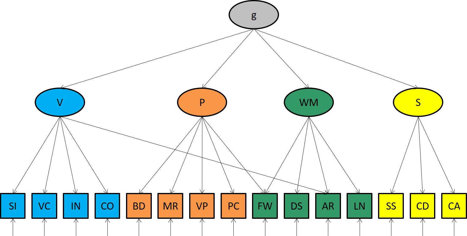
Theoretically, the WAIS-IV measures the following latent traits:
lvars  <- c( "P", # Perceptual
             "V", # Verbal
             "W", # Working Memory
             "S"  # Speed
            )
So 4 in total. In g theory, the variable g explains the correlations among those factors.
ne <- length( lvars )
The pattern of factor loadings is as follows:
lambda_g  <- lambda_b <- matrix( c ( #P  V  W  S  g
                                      1, 0, 0, 0, 0, # BD
                                      0, 1, 0, 0, 0, # SI
                                      0, 0, 1, 0, 0, # DS
                                      1, 0, 0, 0, 0, # MR
                                      0, 1, 0, 0, 0, # VC
                                      0, 1, 1, 0, 0, # AR
                                      0, 0, 0, 1, 0, # SS
                                      1, 0, 0, 0, 0, # VP
                                      0, 1, 0, 0, 0, # IN
                                      0, 0, 0, 1, 0, # CD
                                      0, 0, 1, 0, 0, # LN
                                      1, 0, 1, 0, 0, # FW
                                      0, 1, 0, 0, 0, # CO
                                      0, 0, 0, 1, 0, # CA
                                      1, 0, 0, 0, 0  # PC
                                     ),
                                  ncol = ne + 1,
                                  byrow = TRUE )
In the bifactor model the subtests measure g directly.

lambda_b[ , ne + 1 ] <- 1
Not that this implies that tests are suddenly not unidimensional anymore!
In the higher order factor model, tests remain unidimensional. As mentioned, the correlations bewteen the first order factors are explained by their common dependence on g, the general factor of intelligence.
The pattern of factor loadings on the second level is thus:
# # factor loadings in the second order (in the g model only)
beta_g     <- matrix( c ( #P  V  W  S g
                           0, 0, 0, 0, 1, # P
                           0, 0, 0, 0, 1, # V
                           0, 0, 0, 0, 1, # W
                           0, 0, 0, 0, 1, # S,
                           0, 0, 0, 0, 0  # g
                          ),
                       ncol = ne + 1,
                       byrow = TRUE )
As a result scores on all subtests are all positively intercorrelated. This robust empirical finding is commonly referred to as 'the positive manifold'.
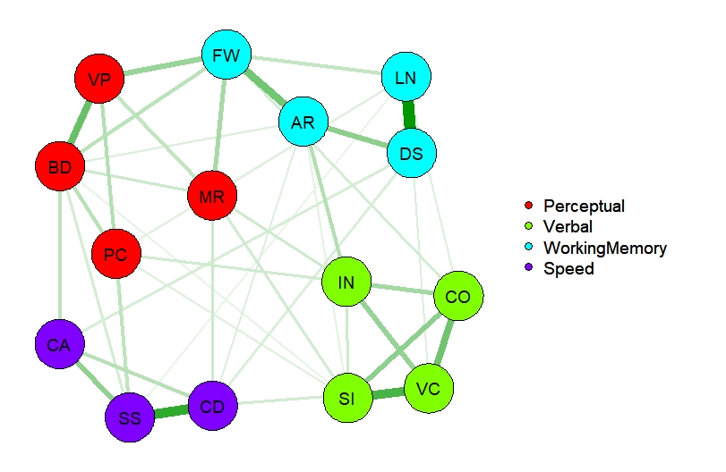
In the network approach, the positive manifold is due to a manifold of positive interactions. No latent variables need to be assumed.
How can we model this? Here's an example of the extraction of a network. Note that this an exploratory analysis.
# Extract a network form the US Sample
NWModel_US <- ggm( covs = ( n_US - 1 )/n_US*WAIS_US,
                   omega = "Full",
                   nobs = n_US )

# Prune it
NWModel_US <- NWModel_US %>% prune( alpha = 0.01, recursive = TRUE )

# Aim for further improvement
NWModel_US <- NWModel_US %>% stepup
However, now we have such a network, we can fit it confirmatory on any other sample (in OpenMx or in Psychonetrics). Here's the pattern of relations.
# Extract the adjacency matrix and use it as confirmatory network in the German sample
omega <- 1*( getmatrix( NWModel_US, "omega" ) !=0 )
Here the aim is to fit all three models on the German standardization sample data. Let's first collect - per model - all important matrices and other pieces of information
# parameters of the Higher Order Factor Model (HF)
paramsHF  <- list( lambda = lambda_g,
                   beta = beta_g,
                   sigma_zeta = 'empty',
                   identification = "variance",
                   type = 'lvm' )

# parameters of the BifFactor Model (BF)
paramsBF  <- list( lambda = lambda_b,
                   sigma_zeta = 'empty',
                   identification = "variance",
                   type = 'lvm' )

# parameters of the Network Model (NW)
paramsNW  <- list( omega = omega,
                   type = 'ggm' )

# Store them in a list
models <- list( HF = paramsHF, BF = paramsBF, NW = paramsNW )
Next actually fit the models on the data. With function lapply, we only need one line of code.
results <- lapply( models, function(i) fitModel( cov, i, n_Germany ) )
The model implied correlations, we will use in the next step, the actual data generation. Let's extract those correlations from the results.
# Extract the model standardized model implied covariance (correlation) matrices
st_sigmas <- lapply( results,
                     function(i) { cov2cor ( matrix( getmatrix( i, "sigma"  ),
                                                     ny, ny, TRUE,
                                                     list( yvars, yvars  ) ) ) } )
In order to make our findings replicatable, we chose the following seed
set.seed( 03012021 ) # start of Tasos' internship
We simulate a 1000 data sets for each model implied correlation matrix.
nrep <- 1000
The sample size is taken the same as the (German) sample size, from which the model implied correlation matrices were extracted.
We are ready to simulate!
simdat <- lapply( st_sigmas,
                  function( sigma ) replicate( nrep,
                                               mvrnorm( n_Germany,
                                                        rep( 0, ny ),
                                                        sigma ) ) )
Fit all (3) models on all (3x1000) data sets. Note: this might take a few hours!
simres <- lapply( models,
                  function( model ) lapply( simdat,
                                            function(i) apply( i,
                                                               3,
                                                               function( dat ) fitModel( dat,
                                                                                         model ) ) ) )
Following Cucina et al. and Kan et al., we will considere the RMSEA, CFI, TLI, NFI, Chi-square statistics, AIC, BIC, and
rmseas  <- extractFitm( simres, 'rmsea'  )
cfis    <- extractFitm( simres, 'cfi'    )
tlis    <- extractFitm( simres, 'tli'    )
nfis    <- extractFitm( simres, 'nfi'    )
chisqs  <- extractFitm( simres, 'chisq'  )
dfs     <- extractFitm( simres, 'df'     )
pvalues <- extractFitm( simres, 'pvalue' )
aics    <- extractFitm( simres, 'aic.ll' )
bics    <- extractFitm( simres, 'bic'    )
dchisqs <- lapply( chisqs, function(i) apply(i, 1, function(i) i$HF-i$BF ) )
ddfs    <- lapply( dfs,    function(i) apply(i, 1, function(i) i$HF-i$BF ) )
ps_diff <- lapply( dchisqs, function(i) 1 - pchisq( i, df = 11 ) )
Let's plot the most important results
histFitm( rmseas )  # near perfect if the fitted model is the true model
histFitm( cfis )    # near perfect if the fitted model is the true model
histFitm( tlis )    # near perfect if the fitted model is the true model
histFitm( nfis )    # near perfect if the fitted model is the true model
histFitm( chisqs )  # distributed around df if the fitted model is the true model
histFitm( pvalues ) # uniformly distributed if the fitted model is the true model
And tabelize them
# tables (do fit measures pick the true model when the true model is included in the comparison )
lapply( rmseas, function(i) table( apply( i, 1, which.min ) ) )
lapply( cfis,   function(i) table( apply( i, 1, which.max ) ) )
lapply( tlis,   function(i) table( apply( i, 1, which.max ) ) )
lapply( nfis,   function(i) table( apply( i, 1, which.max ) ) )
lapply( aics,   function(i) table( apply( i, 1, which.min ) ) )
lapply( bics,   function(i) table( apply( i, 1, which.min ) ) )
What was our hypothesis?
'If the network is the true model but not considered, the bifactor model is preferred over the higher order factor model' ( as a summary of the data )
lapply( rmseas, function(i) table( apply( i[,1:2], 1, which.min ) ) )$NW
lapply( cfis,   function(i) table( apply( i[,1:2], 1, which.max ) ) )$NW
lapply( nfis,   function(i) table( apply( i[,1:2], 1, which.max ) ) )$NW
lapply( aics,   function(i) table( apply( i[,1:2], 1, which.min ) ) )$NW
lapply( bics,   function(i) table( apply( i[,1:2], 1, which.min ) ) )$NW
And what can be expected if the bifactor model would be the true model?
lapply( rmseas, function(i) table( apply( i[,1:2], 1, which.min ) ) )$BF
lapply( cfis,   function(i) table( apply( i[,1:2], 1, which.max ) ) )$BF
lapply( nfis,   function(i) table( apply( i[,1:2], 1, which.max ) ) )$BF
lapply( aics,   function(i) table( apply( i[,1:2], 1, which.min ) ) )$BF
lapply( bics,   function(i) table( apply( i[,1:2], 1, which.min ) ) )$BF
Show in figures
layout( matrix( 1:9, 3, 3, TRUE ) )
hist( ps_diff$HF, main = paste( 'Comparison HF and BF', '\nTrue model = HF' ), xlab = 'P (chisq diff)' )
hist( ps_diff$BF, main = paste( 'Comparison HF and BF', '\nTrue model = BF' ), xlab = 'P (chisq diff)' )
hist( ps_diff$NW, main = paste( 'Comparison HF and BF', '\nTrue model = NW' ), xlab = 'P (chisq diff)' )
In summary:
Absolute fit (chisq): ACCEPT THE MODEL IN 95% OF THE CASES
hist( unlist( pvalues$BF[,'BF'] ), main = paste( 'BF absolute fit',    '\nTrue model = BF'), xlab = 'P (chisq)' )
# approximate fit: NEAR PERFECT
hist( unlist( nfis$BF[,'BF'] ),    main = paste( 'BF approximate fit', '\nTrue model = BF'), xlab = 'nfi' )
# close fit: NEAR PERFECT
hist( unlist( rmseas$BF[,'BF'] ),  main = paste( 'BF close fit',       '\nTrue model = BF'), xlab = 'RMSEA' )

# absolute fit (chisq): reject the model
hist( unlist( pvalues$NW[,'BF'] ), main = paste( 'BF absolute fit',    '\nTrue model = NW'), xlab = 'P (chisq)' )
# approximate fit: good
hist( unlist( nfis$NW[,'BF'] ),    main = paste( 'BF approximate fit', '\nTrue model = NW'), xlab = 'nfi' )
# close fit: acceptable(?)
hist( unlist( rmseas$NW[,'BF'] ),  main = paste( 'BF close fit',       '\nTrue model = NW'), xlab = 'RMSEA' )

The empirical results are more in line with the situation in which the true model is a network model than in the situation in which the true model is a bifactor model!
Epskamp, S. (2021). Psychonetrics. R package. version 0.8.1.
Hood, S. B. (2008). Latent variable realism in psychometrics. Indiana University Press.
Jensen, A. R. (1998). The g factor: The science of mental ability. Westport, CT: Praeger.