The stock market is a focus for investors to maximize their potential profits and consequently, the interest shown from the technical and financial sides in stock market prediction is always on the rise.
However, stock market prediction is a problem known for its challenging nature due to its dependency on diverse factors that affect the market, these factors are unpredictable and cannot be taken into consideration such as political variables, and social media effects such as twitter on the stock market.
- ARIMA is a statistical analysis model that predicts the future of a variable with respect to time or for a better understanding of the time series dataset.
- ARIMA is a generalization of Auto-Regressive, Moving Average, and integration terms. Those terms would be explained briefly in the following section.
- Auto-Regressive (AR): is a specific type of regression model, which means the current values are correlated with previous values in the time steps. To be more precise it’s partial Auto-correlation.
Y(t) = β1 + Ф1 Y(t-1) + Ф2 Y(t-2) +.. + Фp Y(t-p) And, the (P) is the lagged order- Moving Average (MA): is analyzing the errors from the lagged observations and how they affect the current observation.
Y(t) = β2 + 𝟂1 𝞷(t-1) + 𝟂2 𝞷(t-2) +.. + 𝟂p 𝞷(t-p) The 𝞷 terms are the errors observed, the 𝟂 is the weight of this error, and 𝟂 are calculated using a statistical correlation test. And, (q) represents the size of the moving average that has a significant impact on the current observation.- Integrated (I): the previous models can handle only the stationary time series dataset, which has a constant mean (μ), and variance (σ) without having seasonality. By taking the difference between consecutive timesteps, this transform will eliminate the trend and keep the mean constant. So, they defined (d) the order of differencing which means how many times we would apply the differencing process.
Till now, ARIMA can handle Non-stationary data with trends, but can’t handle the seasonality component, So, SARIMA (Seasonal Autoregressive Integrated Moving Average) was introduced as an extension adding more parameters to handle the seasonality.
SARIMA Parameters:
- p: non-seasonal or trend autoregressive (AR) order
- d: non-seasonal or trend differencing
- q: non-seasonal or trend moving average (MA) order
- P: seasonal AR order
- D: seasonal differencing
- Q: seasonal MA order
- S: length of repeating seasonal pattern
To identify the values of AR and MA parameters we use ACF and PACF plots. Or by using grid search to go over all the combinations of parameters and chose the one that achieves the least loss according to a defined loss function such as Akaike Information Criterion (AIC) and Bayesian Information Criterion (BIC) as both are penalized-likelihood information criteria. And to identify the integrated parameters, they use a statistical test called the “Augmented Dickey-Fuller test”
- Note: Due to the headache of identifying the model and its parameters, the python community has developed an automated library called “Auto Arima” that chooses the best model suitable for your dataset and identifies the best parameters to achieve the lowest loss.
Convolutional Neural Networks (CNN):
The 1-d convolutional neural networks are used intensively in time series forecasting for a fixed window length, CNN has the ability to remove the noise and unrelated patterns along the time series data. Also, the convolutional and pooling layers both perform smoothing to the data instead of the traditional weighted average with require manual tuning.
Convolution learn from data through its filter’s weights update. CNN layers depend on the learning of the filters, so these filters after training will be able to detect the features.
The pooling layer mainly smooths out and reduces the local noise by averaging the time series values.
The data change after each layer:
Figure 1: the change due to the CNN layer
Figure 2: the change due to the pooling layer
LSTM (Long Short-Term Memory) networks have the ability to learn long-term dependencies, especially, in a sequence prediction problem as time series, LSTM has outstanding performance on a large variety of data.

Important Note: The Bidirectional LSTM can learn in both direction forward and backward sequences, also the Bidirectional has complete information about all the points in the data.
- Stock Data Scraping
- Twitter Data Scraping
- Twitter Data Preprocessing and Sentiment analysis
- Modeling Using Two approaches
- ARIMA as Baseline
- Deep learning architecture using 1D-CNN and BiCudaLSTM layers as our new approach
- Compare and evaluate our approach vs ARIMA
- Evaluate our approach against new data in real-time
-
The Stock Data: The research team downloaded the stock data of Netflix in Spreadsheet from Yahoo Finance website from Jan 1st, 2018 to July 7th, 2022
-
The Twitter Data: The research team scrapped within the same period using the Snscrape tool.
Note: Twitter API could not be used in this project as it was limited to only one week
After scrapping the tweets, it was uncleaned text. So, we go through a cleaning process as shown:
- Lowering the sentences.
- Removing the attached links, hashtags, symbols, and numerical values.
- Translate emojis into their meanings.
- Tokenize sentences by Twitter.
- Removing stop Words and punctuations
- Applying lemmatization on each word.
As the volume of tweets was huge, it was a challenge to label them manually, so the research team used a pre-trained model called “twitter-slm-roberta-base-sentiment” which was trained on 198 million tweets to get the polarity of each tweet.
The polarity score was converted into three values;1, 0, and -1 for each class as 1 represents a positive tweet, 0 represents a neutral tweet, and -1 represents a negative tweet.
> Due to each day having 350 tweets on average, it was aggregated by the average of polarities to get only a single number per day.
the polarities were combined with the stock data to form one dataset to be used in time series models.

The input of the library should be in the form of y (predicted output) and X (features) as shown:
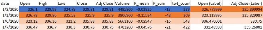
Open, High, Low, Close, Adj Close, Volume, P_mean, P_sum, twt_count should be mapped to the Open and Close of the next data to be considered as the prediction.
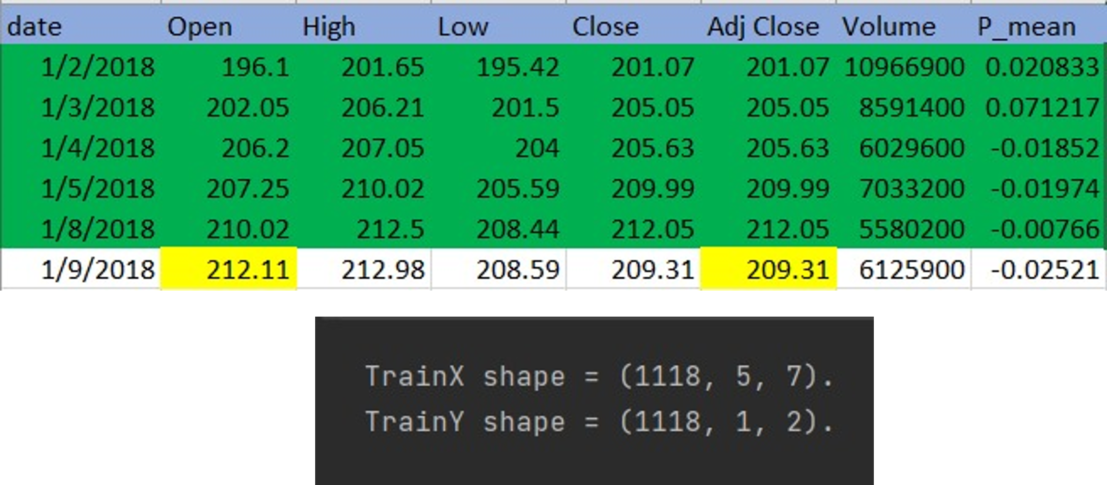
In the time series problems with deep learning, the dataset should be reshaped to features and the target. The features consist of the number of previous days we look at and the target consists of the predicted future days and the number of predicted features. The dataset for this project is 1128 samples and the look-back days are 5 days, and the number of features is 7, so the features will be reshaped to (1118,5,7) and if the number of future days is 1 and the predicted features are 2 so the shape will be (1118,1,2). The shape of features without the Twitter sentiment analysis is (1118,5,6). The last 5 days were dropped because they don’t have target value.
Due to the headache of identifying the model and its parameters, the python community has developed an automated library called “Auto Arima” that chooses the best model suitable for your dataset and identifies the best parameters to achieve the lowest loss. Our arima model is architecture:
Our CNN-LSTM model Architecture with time series problems which consist of a CNN block followed by an LSTM block and finally fully connected layers as shown in the figure below.

This combination of using CNN and LSTM increased the accuracy instead of using only LSTM or CNN. The use of the CNN at first makes the model able to extract the features of the data and then the LSTM block saves the sequence of the data. The use of CUDNN-LSTM layers instead of the original LSTM layers makes the training very fast as the time is reduced to approximately 3x.
While we compared the results of the two models we found:
- The tweets have a positive impact as the accuracy increased.
- Our model has a fast-learning curve, which achieved the Arima's accuracy in a few epochs, and without much optimization effort
- expected to have a better performance if the model trained, again with more data and with more tuning to the parameter. taking into consideration that LSTM and CNN when getting more data would learn significantly.
Run the following command:
$ pip3 install git+https://github.com/JustAnotherArchivist/snscrape.git
Then using the following python lines:
import os
text_query = "$NFLX" # specify the company you need $NFLX = Netflix company
since_date = "2018-01-01" # specify the start date
until_date = "2022-07-11" # specify the end date
os.system('snscrape --jsonl --since {} twitter-search "{} until:{}"> text-query-tweets.json'.format(since_date, text_query, until_date))Run the following command:
$ pip install transformers
$ pip install transformers[sentencepiece]
from transformers import TFAutoModelForSequenceClassification
from transformers import AutoTokenizer, AutoConfig

MODEL = f"cardiffnlp/twitter-xlm-roberta-base-sentiment"

tokenizer = AutoTokenizer.from_pretrained(MODEL)
config = AutoConfig.from_pretrained(MODEL)

# After loading the models you can use them
model = TFAutoModelForSequenceClassification.from_pretrained(MODEL)
model.save_pretrained(MODEL)
tokenizer.save_pretrained(MODEL)

encoded_input = tokenizer(input_text, return_tensors='tf')
final_output = model(encoded_input)- LSTM-CNN prediction implemented paper:
- The sentiment analysis model (twitter-slm-roberta-base-sentiment)