inputs = Input()

z = Conv2D(input_shape=(224, 224, 3), filters=64, kernel_size=(3, 3), padding="same", activation="relu")(inputs)
z = Conv2D(filters=64, kernel_size=(3, 3), padding="same", activation="relu")(z)
z = MaxPool2D(pool_size=(2, 2), strides=(2, 2)(z))
z = Conv2D(filters=128, kernel_size=(3, 3), padding="same", activation="relu")(z)
z = Conv2D(filters=128, kernel_size=(3, 3), padding="same", activation="relu")(z)
z = MaxPool2D(pool_size=(2, 2), strides=(2, 2)(z))
z = Conv2D(filters=256, kernel_size=(3, 3), padding="same", activation="relu")(z)
z = Conv2D(filters=256, kernel_size=(3, 3), padding="same", activation="relu")(z)
z = Conv2D(filters=256, kernel_size=(3, 3), padding="same", activation="relu")(z)
z = MaxPool2D(pool_size=(2, 2),strides=(2, 2)(z))
z = Conv2D(filters=512, kernel_size=(3, 3), padding="same", activation="relu")(z)
z = Conv2D(filters=512, kernel_size=(3, 3), padding="same", activation="relu")(z)
z = Conv2D(filters=512, kernel_size=(3, 3), padding="same", activation="relu")(z)
z = MaxPool2D(pool_size=(2, 2),strides=(2, 2)(z))
z = Conv2D(filters=512, kernel_size=(3, 3), padding="same", activation="relu")(z)
z = Conv2D(filters=512, kernel_size=(3, 3), padding="same", activation="relu")(z)
z = Conv2D(filters=512, kernel_size=(3, 3), padding="same", activation="relu")(z)
z = MaxPool2D(pool_size=(2, 2),strides=(2, 2)(z))
z = Flatten()(z)
z = Dense(units=4096, activation="relu")(z)
z = Dense(units=4096, activation="relu")(z)

outputs = Dense(units=2, activation="softmax")(z)- Paper: https://www.cs.unc.edu/~wliu/papers/GoogLeNet.pdf
- Source: https://www.geeksforgeeks.org/understanding-googlenet-model-cnn-architecture/
- The novel architecture was an Inception Network, and a variant of this Network called, GoogLeNet went on to achieve the state of the art performance in the classification computer vision task of the ImageNet LargeScale Visual Recognition Challenge 2014(ILVRC14).
- Global Average Pooling (GAP)
- This also decreases the number of trainable parameters to 0 and improves the top-1 accuracy by 0.6%.
- Auxiliary Classifier for Training:
- Inception architecture used some intermediate classifier branches in the middle of the architecture, these branches are used during training only. These branches consist of a 5×5 average pooling layer with a stride of 3, a 1×1 convolutions with 128 filters, two fully connected layers of 1024 outputs and 1000 outputs and a softmax classification layer. The generated loss of these layers added to total loss with a weight of 0.3. These layers help in combating gradient vanishing problem and also provide regularization.
- Two auxiliary classifier layer connected to the output of Inception (4a) and Inception (4d) layers.
- Implementation
 def auxiliary_classifier(x, name):
 	z = AveragePooling2D(pool_size=5, strides=3, padding="valid")(x)
 	z = Conv2D(filters=128, kernel_size=1, strides=1, padding="same", activation="relu")(z)
 	z = Flatten()(z)
 	z = Dense(units=1024, activation="relu")(z)

 	return Dense(units=1000, activation="softmax", name=name)(z)
- Sources: https://towardsdatascience.com/deep-learning-understand-the-inception-module-56146866e652, https://hacktildawn.com/2016/09/25/inception-modules-explained-and-implemented/
- An inception network is a deep neural network with an architectural design that consists of repeating components referred to as Inception modules.
- Convolutional neural networks benefit from extracting features at varying scales. The biological human visual cortex functions by identifying patterns at different scales, which accumulates to form lager perceptions of objects. Therefore multi-scale convnet have the potential to learn more. Large networks are prone to overfitting, and chaining multiple convolutional operations together increases the computational cost of the network.
- Although a 1x1 filter does not learn any spatial patterns that occur within the image, it does learn patterns across the depth(cross channel) of the image. 1x1 convolutions reduce the dimensions of inputs within the network. 1x1 convolutions are configured to have a reduced amount of filters, so the outputs typically have a reduced amount of channels in comparison to the initial input.
- Within a convnet, different conv filter sizes learn spatial patterns and detect features at varying scales.
- 1x1 learns patterns across the depth of the input. 3x3 and 5x5 learns spatial patterns across all dimensional components (height, width and depth) of the input.
- There is an increase in representational power when combining all the patterns learned from the varying filter sizes. The Inception module consists of a concatenation layer, where all the outputs and feature maps from the conv filters are combined into one object to create a single output of the Inception module.
- Naive Inception Module
- Pooling downsamples the input data to create a smaller output with a reduced height and width.
- Within an Inception module, we add padding(same) to the max-pooling layer to ensure it maintains the height and width as the other outputs(feature maps) of the convolutional layers within the same Inception module. By doing this, we ensure we can concatenate the outputs of the max-pooling layer with the outputs of the conv layers within the concatenation layer.
- Implementation
 def naive_inception_module(x, filters):
 	z1 = Conv2D(filters=filters[0], kernel_size=1, strides=1, padding="same", activation="relu")(x)
 	z2 = Conv2D(filters=filters[1], kernel_size=3, strides=1, padding="same", activation="relu")(x)
 	z3 = Conv2D(filters=filters[2], kernel_size=5, strides=1, padding="same", activation="relu")(x)
 	z4 = MaxPool2D(pool_size=3, strides=1, padding="same")(x)
 	return Concatenate(axis=-1)([z1, z2, z3, z4])
- Inception Module
- Implementation
 def inception_module(x, filters):
 	z1 = Conv2D(filters=filters[0], kernel_size=1, strides=1, padding="same", activation="relu")(x)

 	z2 = Conv2D(filters=filters[3], kernel_size=1, strides=1, padding="same", activation="relu")(x)
 	z2 = Conv2D(filters=filters[1], kernel_size=3, strides=1, padding="same", activation="relu")(z2)

 	z3 = Conv2D(filters=filters[3], kernel_size=1, strides=1, padding="same", activation="relu")(x)
 	z3 = Conv2D(filters=filters[2], kernel_size=5, strides=1, padding="same", activation="relu")(z3)

 	z4 = MaxPool2D(pool_size=3, strides=1, padding="same")(x)
 	z4 = Conv2D(filters=filters[3], kernel_size=1, strides=1, padding="same", activation="relu")(z4)
 	return Concatenate(axis=-1)([z1, z2, z3, z4])
- Implementation
 inputs = Input(shape=(224, 224, 3))

 z = Conv2D(filters=64, kernel_size=7, strides=2, padding="same", activation="relu")(inputs)
 z = MaxPool2D(pool_size=3, strides=2, padding="same")(z)
 z = BatchNormalization()(z)
 z = Conv2D(filters=64, kernel_size=1, strides=1, padding="same", activation="relu")(z)
 z = Conv2D(filters=192, kernel_size=3, strides=1, padding="same", activation="relu")(z)
 z = BatchNormalization()(z)
 z = MaxPool2D(pool_size=3, strides=2, padding="same")(z)
 z = inception_module(z, [64, 128, 32, 32]) # inception 3a
 z = inception_module(z, [128, 192, 96, 64]) # inception 3b
 z = MaxPool2D(pool_size=3, strides=2, padding="same")(z)
 z = inception_module(z, [192, 208, 48, 64]) # inception 4a

 outputs1 = auxiliary_classifier(z, "outputs1")

 z = inception_module(z, [160, 224, 64, 64]) # inception 4b
 z = inception_module(z, [128, 256, 64, 64]) # inception 4c
 z = inception_module(z, [112, 288, 64, 64]) # inception 4d

 outputs2 = auxiliary_classifier(z, "outputs2")

 z = inception_module(z, [256, 320, 128, 128]) # inception 4e
 z = MaxPool2D(pool_size=3, strides=2, padding="same")(z)
 z = inception_module(z, [256, 320, 128, 128]) # inception 5a
 z = inception_module(z, [384, 384, 128, 128]) # inception 5b
 z = GlobalAveragePooling2D()(z)
 z = Dropout(rate=0.4)(z)
 z = Flatten()(z)

 outputs3 = Dense(units=1000, activation="softmax")(z)

 model = Model(inputs=inputs, outputs=[outputs1, outputs2, outputs3])


- Source: https://en.wikipedia.org/wiki/Residual_neural_network, https://www.analyticsvidhya.com/blog/2021/08/all-you-need-to-know-about-skip-connections/#:~:text=Skip%20Connections%20(or%20Shortcut%20Connections,input%20to%20the%20next%20layers.&text=Neural%20networks%20can%20learn%20any,%2Ddimensional%20and%20non%2Dconvex, https://www.analyticsvidhya.com/blog/2021/06/understanding-resnet-and-analyzing-various-models-on-the-cifar-10-dataset/#h2_3
- Residual Networks were proposed in 2015 to solve the image classification problem. ****In ResNets, the information from the initial layers is passed to deeper layers by matrix addition. This operation doesn’t have any additional parameters as the output from the previous layer is added to the layer ahead.
- There are two main reasons to add skip connections: to avoid the problem of vanishing gradients, or to mitigate the Degradation (accuracy saturation) problem; where adding more layers to a suitably deep model leads to higher training error.
- Skipping effectively simplifies the network, using fewer layers in the initial training stages. This speeds learning by reducing the impact of vanishing gradients, as there are fewer layers to propagate through.
- While training deep neural nets, the performance of the model drops down with the increase in depth of the architecture. This is known as the degradation problem.
- From this construction, the deeper network should not produce any higher training error than its shallow counterpart because we are actually using the shallow model’s weight in the deeper network with added identity layers. But experiments prove that the deeper network produces high training error comparing to the shallow one. This states the inability of deeper layers to learn even identity mappings.
- The degradation of training accuracy indicates that not all systems are similarly easy to optimize.
- One of the primary reasons is due to random initialization of weights with a mean around zero, L1, and L2 regularization. As a result, the weights in the model would always be around zero and thus the deeper layers can’t learn identity mappings as well. Here comes the concept of skip connections which would enable us to train very deep neural networks.
- Skip Connections (or Shortcut Connections) as the name suggests skips some of the layers in the neural network and feeds the output of one layer as the input to the next layers.
- Skip Connections were introduced to solve different problems in different architectures. In the case of ResNets, skip connections solved the degradation problem that we addressed earlier.
- As you can see here, the loss surface of the neural network with skip connections is smoother and thus leading to faster convergence than the network without any skip connections.
- Skip Connections can be used in 2 fundamental ways in Neural Networks: Addition and Concatenation.
- One problem that may happen is regarding the dimensions. Sometimes the dimensions of
xandF(x)may vary and this needs to be solved. Two approaches can be followed in such situations. One involves padding the input x with weights such as it now brought equal to that of the value coming out. The second way includes using a convolutional layer fromxto addition toF(x).
- Source: https://towardsdatascience.com/review-resnet-winner-of-ilsvrc-2015-image-classification-localization-detection-e39402bfa5d8
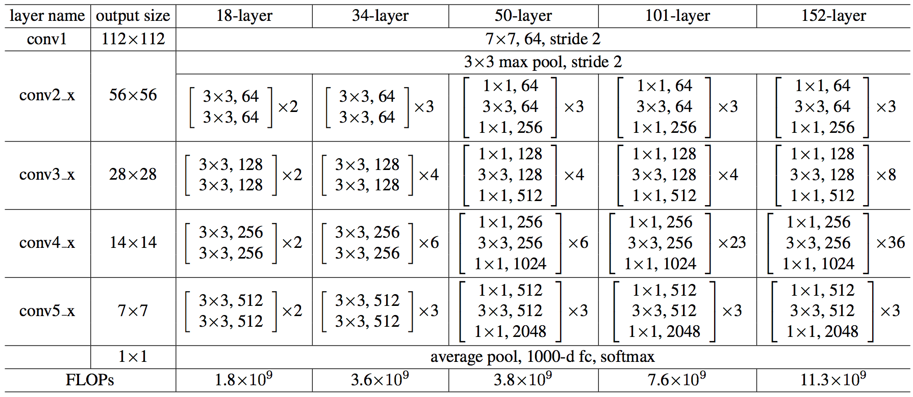
- Since the network is very deep now, the time complexity is high. A bottleneck design is used to reduce the complexity.
- The 1×1 conv layers are added to the start and end of network. This is a technique suggested in Network In Network and GoogLeNet (Inception-v1). It turns out that 1×1 conv can reduce the number of connections (parameters) while not degrading the performance of the network so much. (Please visit my review if interested.)
- With the bottleneck design, 34-layer ResNet become 50-layer ResNet. And there are deeper network with the bottleneck design: ResNet-101 and ResNet-152.
- Implementation of 50-layered ResNet (for CIFAR-10)
 def residual_block(x, filters):
 	z1 = Conv2D(filters=filters[0], kernel_size=1, strides=1, padding="same")(x)
 	z1 = BatchNormalization()(z1)
 	z1 = Activation("relu")(z1)
 	z1 = Conv2D(filters=filters[0], kernel_size=3, strides=1, padding="same")(z1)
 	z1 = BatchNormalization()(z1)
 	z1 = Activation("relu")(z1)
 	z1 = Conv2D(filters=filters[1], kernel_size=1, strides=1, padding="same")(z1)
 	z1 = BatchNormalization()(z1)
 	z1 = Activation("relu")(z1)

 	z2 = Conv2D(filters=filters[1], kernel_size=1, strides=1, padding="same")(x)
 	z2 = BatchNormalization()(z2)

 	z = Activation("relu")(z1 + z2)
 	return z

 inputs = Input(shape=(32, 32, 3))

 z = Conv2D(filters=64, kernel_size=7, strides=2, padding="valid")(inputs)
 z = MaxPool2D(pool_size=3, strides=2, padding="same")(z)
 for _ in range(3):
 	z = residual_block(z, filters=[64, 256])
 for _ in range(4):
 	z = residual_block(z, filters=[128, 512])
 for _ in range(6):
 	z = residual_block(z, filters=[256, 1024])
 for _ in range(3):
 	z = residual_block(z, filters=[512, 2048])
 z = GlobalAveragePooling2D()(z)

 outputs = Dense(units=10, activation="softmax")(z)

 model = Model(inputs=inputs, outputs=outputs)
- Source: https://towardsdatascience.com/squeeze-and-excitation-networks-9ef5e71eacd7
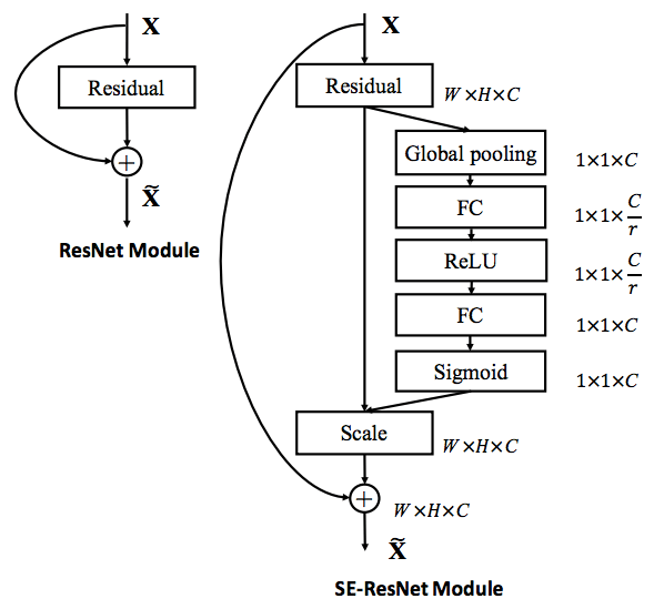
- Squeeze-and-Excitation Networks (SENets) introduce a building block for CNNs that improves channel interdependencies at almost no computational cost. Besides this huge performance boost, they can be easily added to existing architectures. The main idea is this: Let’s add parameters to each channel of a convolutional block so that the network can adaptively adjust the weighting of each feature map.
- CNNs use their convolutional filters to extract hierarchal information from images. Lower layers find trivial pieces of context like edges or high frequencies, while upper layers can detect faces, text or other complex geometrical shapes. They extract whatever is necessary to solve a task efficiently.
- All you need to understand for now is that the network weights each of its channels equally when creating the output feature maps. SENets are all about changing this by adding a content aware mechanism to weight each channel adaptively. In it’s most basic form this could mean adding a single parameter to each channel and giving it a linear scalar how relevant each one is.
- First, they get a global understanding of each channel by squeezing the feature maps to a single numeric value. This results in a vector of size n, where n is equal to the number of convolutional channels. Afterwards, it is fed through a two-layer neural network, which outputs a vector of the same size. These n values can now be used as weights on the original features maps, scaling each channel based on its importance.
- Implementation
 def se_block(x, c, r=16):
 	z = GlobalAveragePooling2D()(x)
     z = Dense(units=c//r, activation="relu")(z)
     z = Dense(units=c, activation="sigmoid")(z)
     return z*x