As all our team members are international students living outside the campus and do not own any car. Therefore, the school bus has been our main transportation tool, the bus line which is called “South City Line”. The original route of the “South City Line” is from the campus to Mutiara Residence, Univ360 Residence, South City Plaza, East Lake Residence, Sky Villa Residence, KTM Serdang, and turn back to the campus. It is believed that all the bus takers have experienced the traffic jam during the route around South City Plaza. Generally, there are certain number of international students are living near to the KTM Serdang, The Mines Resort, the traffic jam of the route from the campus to KTM Serdang is not heavy, and we can find it when we take the Grab ride. Moreover, there is a Free Bus line of Rapid KL called “SJ04”, which is covering the route from KTM Serdang to our campus, and it is our second plan to travel from home to campus, the passengers can tell the driver what their destinations are, and the driver can adjust the route by themselves. The drivers would love to avoid the route around South City Plaza to avoid the terrible traffic jam. The action the drivers took really inspired us, and we decide to do some improvements.

Figure 1 “South City” bus line schedule
The Traveling Salesman Problem (TSP) is an NP-hard problem. In computational complexity theory, NP stands for "nondeterministic polynomial time", which means that the time required to solve the problem using a non-deterministic algorithm is polynomial in the size of the input. NP-hard problems are a class of problems that are at least as difficult as the hardest problems in NP, meaning that if any NP-hard problem can be solved efficiently, then all problems in NP can be solved efficiently as well. Therefore, TSP is considered to be one of the most difficult problems in computer science. I will provide an example of TSP as an NP-complete problem using a map for university bus travelling problem.
As Figure 1 shown above, we were thinking about developing an application base on the timetable; Assuming that the bus is going to departure at 7:15am for the first roll, the reservation function will be activated 1 hour before the departure of the bus. The application will store the information of the “calling” stations and only travel around the “called” stations. It is not guaranteed that the traffic jam will be avoided every roll, but it is optimistic to avoid it some of the times.
Finding an optimal solution for this scenario is important for several reasons.
Improved punctuality: By allowing users to schedule appointments for their bus rides, the bus routes can be optimized to reduce the amount of time spent in traffic. This means that students and staff will be able to arrive on campus in a timelier manner.
Increased efficiency: By optimizing the bus routes, the number of buses needed to transport students and staff can be reduced, which will save time, fuel, and money.
Increased safety: By reducing the amount of time spent in traffic, the risk of accidents caused by traffic congestion is also reduced.
Enhanced student and staff satisfaction: When students and staff can arrive on campus in a timely manner, they will be more satisfied with the bus service. This can lead to improved morale and motivation among students and staff.
Better university image: When the bus service is efficient, punctual, and safe, the university will be viewed more favorably by prospective students and their parents, as well as by staff and faculty members.
Cost Savings: The bus service is a major cost for the university and making it more efficient, can also reduce the cost of the service.
In summary, finding an optimal solution for this scenario is crucial to improve the overall transportation experience for the university community and to enhance the university's image.
Sorting algorithm:
Strengths: efficient for small data sets and able to handle simple data structures
Weaknesses: Not suitable for solving the problem of optimizing bus routes as it does not guarantee the shortest route and not designed to solve the traveling salesman problem.
Divide and Conquer (DAC):
Strengths: Can be used to divide the problem into smaller subproblems and solve them independently, which can make the problem more manageable.
Weaknesses: It may not be able to find the optimal solution for the entire problem, due to the nature of the problem it might become computationally expensive and can lead to a high time complexity.
Dynamic Programming (DP):
Strengths: Can be used to find the optimal solution for the problem by breaking it down into smaller subproblems and storing the solutions for future use.
Weaknesses: It can be computationally expensive for large data sets and can lead to a high time complexity.
Greedy Algorithm:
Strengths: Can be used to find a solution by making locally optimal choices at each step, which can make the problem more manageable.
Weaknesses: It may not guarantee a globally optimal solution, and the solution can be heavily influenced by the initial state.
Graph Algorithm:
Strengths: Graph algorithms such as Dijkstra's algorithm or Bellman-Ford algorithm can be used to find the shortest path between two stops.
Weaknesses: They are not well suited for solving the TSP problem, they are designed to solve a single-source shortest path problem and not the problem of finding the shortest route that visits a set of locations and returns to the starting point.
In conclusion, TSP algorithm is the most appropriate solution paradigm for this problem as it is specifically designed to solve the problem of finding the shortest route that visits a set of locations and returns to the starting point. Other algorithms such as sorting, DAC, DP, greedy and graph algorithms can also be considered but they may not be able to find the optimal solution for this problem and may come with computational limitations.
The algorithm that we have chosen to solve this problem is the classical TSP algorithm also known as the "brute-force" algorithm. The idea behind this algorithm is to generate all possible routes and then select the one with the shortest distance.
The Traveling Salesman Problem (TSP) algorithm is a popular choice for bus route generation because it is a well-established algorithm that can quickly find the optimal route given a set of locations. TSP is an NP-hard problem, which means that it is computationally difficult to find the exact solution in a reasonable amount of time for large sets of data.
Brute force is a method of solving TSP by systematically checking every possible route and selecting the one with the shortest total distance. This approach is very computationally intensive and can become infeasible for large numbers of locations. However, it is a simple and effective method for small sets of data, or as a reference point to compare the results of other algorithms.
The brute force method is not the best choice for large number of location, so it can be used as a reference point to compare the results of other algorithms. Heuristic algorithms such as nearest neighbour, 2-opt, and simulated annealing can also be used to solve TSP problem, which are faster than brute force method.
The selected algorithm can be broken down into the following steps:
1. Initialize an empty list to store all possible routes
2. Generate all possible routes starting from the first bus stop and visiting all other bus stops exactly once.
3. For each route, calculate the total distance traveled.
4. Select the route with the shortest distance as the optimal route.
The algorithm is a recursive one and it is based on the concept of backtracking.
1. Recursive function is called with the current vertex and the remaining set of vertices to be visited.
2. The function generates all possible routes by visiting the remaining vertices and for each route, it calculates the total distance traveled.
3. If all the vertices have been visited, the function returns the route with the shortest distance as the optimal route.
The optimization function of this algorithm is the calculation of the total distance traveled for each route. This function is used to compare the different routes and select the one with the shortest distance.
Given a set of bus stops, find the shortest route that visits all the stops and returns to the starting point.
Input: A list of bus stops, including their coordinates and the distances between each pair of stops.
Output: A list of bus stops in the order they should be visited to form the shortest route.
Constraints: The bus must visit all stops exactly once and return to the starting point.
This problem definition provides a clear and precise understanding of the problem that the algorithm is meant to solve, and what the inputs and outputs of the algorithm should be. It also lays out the constraints that the algorithm needs to consider when finding a solution.

Figure 2 The stations stated on the Google Maps
As the Figure 2 shown above, are the stations that the settled bus line will travel. Since the algorithm that we decided to implement is TSP, therefore we need to collect the distances of every destination to each destination. Then, we extract the abstract graph with the distances that calculated by the Google Maps stated as the figure shown below.

Figure 3 The extracted graph with the distance in meter
The default starting point is setting as FSKTM and be the ending point. The core thought of TSP algorithm is to travel all the node and finally go back to the starting point. The red lines indicate that the route between the 2 stations is likely to experience the traffic jam. The green lines denotes that the route is hardly experienced the traffic jam.
The data structure will be Array List and store the stops information that conclude the distance from this stop to others. The basic data structure will be initialized as below in the format of binary array:
        return new int[][]{
 //             FSKTM   MUTIARA 360     SC      EL      SKY     KTM     SPE
 //	 	0  	1       2 	3  	4 	5 	6 	7
/*0*/	{	0, 	4400,	3800,	5100,	5600,	6500,	5900,	650}, //FSKTM, the start point will always be 1
/*1*/	{	4000,	0,	1000,	2100,	3000,	3900,	6000,	4200},//MUTIARA
/*2*/	{	4300,	1100,	0,	3100,	3500,	4400,	6500,	3100},//360
/*3*/	{	5100,	1600,	1800,	0,	1500,	1500,	4300,	4600},//SC
/*4*/	{	5600,	2900,	3500,	1400,	0,	1000,	4400,	5100},//EL
/*5*/	{	6500,	3800,	4100,	1300,	1000,	0,	2600,	8100},//OS/SKY
/*6*/	{	4100,	2700,	3000,	2200,	2700,	2600,	0,	6000},//KTM
/*7*/	{	6500,	2600,	3100,	4000,	5100,	2600,	5300,	0   },//SPE
        };
    }
The Array that contains the distance and the indexes of the stops
The TSP can be formulated as an integer linear program. Several formulations are known. Two notable formulations are the Miller–Tucker–Zemlin (MTZ) formulation and the Dantzig–Fulkerson–Johnson (DFJ) formulation. The DFJ formulation is stronger, though the MTZ formulation is still useful in certain settings.
Common to both these formulations is that one labels the cities with the numbers 1,……,n and takes Cij > 0 to be the cost (distance) from city i to city j. The main variables in the formulations are:

It is because these are 0/1 variables that the formulations become integer programs; all other constraints are purely linear. In particular, the objective in the program is to minimize the tour length:

Without further constraints, the  will however effectively range over all subsets of the set of edges, which is very far from the sets of edges in a tour and allows for a trivial minimum where all Xij = 0. Therefore, both formulations also have the constraints that there at each vertex is exactly one incoming edge and one outgoing edge, which may be expressed as the 2n linear equations.

These ensure that the chosen set of edges locally looks like that of a tour, but still allow for solutions violating the global requirement that there is one tour which visits all vertices, as the edges chosen could make up several tours each visiting only a subset of the vertices; arguably it is this global requirement that makes TSP a hard problem. The MTZ and DFJ formulations differ in how they express this final requirement as linear constraints.
The TSP algorithm is a recursive algorithm that generates all possible routes and then selects the one with the shortest distance as the optimal route.
1. The TSP function takes in a graph as input, and initializes an empty list to store all possible routes.
2. It then calls the generate_routes function, passing in the graph, an empty route, the current vertex, and the list of routes.
3. The generate_routes function uses a backtracking approach to generate all possible routes by visiting the remaining vertices and adding them to the current route.
4. If all the vertices have been visited, the function adds the route to the list of routes and returns.
5. The TSP function then calls the select_optimal_route function, passing in the list of routes.
6. The select_optimal_route function iterates over the routes and calculates the distance of each route using the calculate_distance function.
7. It compares the distance of each route to the shortest distance and updates the optimal route and the shortest distance if the current route has a shorter distance.
8. Finally, the select_optimal_route function returns the optimal route.
Below is the pseudocode implementation.
TSP(Graph g)
{
    // Initialize an empty list to store all possible routes
    routes = []

    // Generate all possible routes
    generate_routes(g, [], 0, routes)

    // Select the route with the shortest distance as the optimal route
    optimal_route = select_optimal_route(routes)

    return optimal_route
}

generate_routes(Graph g, route, current_vertex, routes)
{
    // Base case: If all vertices have been visited
    if(route contains all vertices in g)
    {
        // Add the route to the list of routes
        routes.append(route)
        return
    }

    // Recursive case: visit the remaining vertices
    for each vertex v in g
    {
        if v is not in route
        {
            // Add vertex v to the current route
            route.append(v)

            // Recursively generate routes
            generate_routes(g, route, v, routes)

            // Remove vertex v from the current route
            route.pop()
        }
    }
}

select_optimal_route(routes)
{
    // Initialize the optimal route to the first route
    optimal_route = routes[0]

    // Initialize the shortest distance to the distance of the first route
    shortest_distance = calculate_distance(optimal_route)

    // Iterate over the remaining routes
    for i = 1 to routes.length
    {
        // Calculate the distance of the current route
        distance = calculate_distance(routes[i])

        // Compare the distance of the current route to the shortest distance
        if(distance < shortest_distance)
        {
            // Update the optimal route and the shortest distance
            optimal_route = routes[i]
            shortest_distance = distance
        }
    }

    return optimal_route
}In order to satisfy the requirements of our bus route designing problem, we need to modify the TSP algorithm to apply the algorithm in Java.
This code shows the procedure of the initialization of the data structures and the instance. The variables of the data structure need to be sign as the specific value. As we mentioned before. For example, the graph will be extracted as a binary array. The best paths will be stored in an Integer List.
public class TSP {
    // 小区数量
    //the number of destinations
    private int cityNum;
    // 距离矩阵
    //graph
    private int[][] distance;
    // 最优路径
    //best path
    private List<Integer> bestPath;
    // 最优距离
    //shortest distance
    private int bestDistance;

    public TSP(int cityNum, int[][] distance) {
        this.cityNum = cityNum;
        this.distance = distance;
        this.bestPath = new ArrayList<>();
        this.bestDistance = Integer.MAX_VALUE;
    }

    public void tsp() {
        // 初始化最优路径
        //initialize the best path
        bestPath.add(0);
        // 从小区0开始旅行
        //start from the first residence or stop
        travel(0, 1, 0, bestPath);
    }

    private void travel(int city, int n, int dis, List<Integer> path) {
        // 所有小区都已经访问过
        //check if all the stop is visited
        if (n == cityNum) {
            // 加上最后一次旅行的距离
            //plu the last distance
            dis += distance[city][0];
            // 更新最优解
            //update the best solution
            if (dis < bestDistance) {
                bestDistance = dis;
                bestPath = new ArrayList<>(path);
                bestPath.add(0);
            }
            return;
        }
// 遍历其他所有小区
        //traversal all the other destinations
        for (int i = 0; i < cityNum; i++) {
// 当前小区已经访问过,跳过
            //if visited, skip
            if (path.contains(i)) {
                continue;
            }
// 加上当前城市到下一个小区的距离
            //add on the distance till the next stop
            int newDis = dis + distance[city][i];
// 剪枝:如果当前距离已经大于已知的最优距离,则无需继续搜索
            //pruning
            if (newDis >= bestDistance) {
                continue;
            }
// 将当前城市加入路径
            //add the current destination to the path
            path.add(i);
// 继续旅行
            //keep travelling
            travel(i, n + 1, newDis, path);
// 回溯
            //recall
            path.remove(path.size() - 1);
        }
    }

    public List<Integer> getBestPath() {
        return bestPath;
    }

    public int getBestDistance() {
        return bestDistance;
    }
1. Firstly, the calling of the algorithm is beginning with the method “tsp()”, we consider it as the “trigger” of this algorithm. It adds the first stop (index “0”) to the bestPath List, and then call the “travel()” method. The values included inside this method are: index of the stops, count number of the recursive, total distance, the path that have traveled for one execution.
2. The “If” statement is to check the count number of the recursive is equal to the total number or not, if so, it will be added on the distance of “last” travel. Moreover, if the total distance at that time is smaller than the bestDistance that will be accumulate in the following code, the best distance will be updated to the total distance at this time, and simultaneously, the bestPath List will be updated be the path that last travel has been. This inner “If” statement we consider as the terminating statement.
3. To traversal all the other stops, and if the path has visited one of the stops, it will skip this stop. Then, add on the distance from the starting stop to the stop in current loop execution. If the current distance is larger than the best distance that has been calculated, then no need further searching.
4. However, if the city is not visited and the current distance is not larger than the pervious distance, the program will add this path as the potential best path, then keep on travelling by calling the travel method again with the value of: current index of the city, the count number of the recursive + 1, the distance from the current stop to the next stop, and the potential best path.
5. path.remove(path.size() - 1) is for the recalling purpose, if the all the recursive execution is terminated.
After the implementation of the graph that we extracted, the result is below:
------Request pick-up:1, no:0------
   ---Default Start Point: FSKTM---
Mutiara Residence: 1
Univ 360 Residence: 1
South City Plaza: 0
East Lake Residence: 0
Skyvilla Residence: 1
KTM Serdang: 1
SPE: 0
Bus Parking Square -> Mutiara Residence -> Univ 360 Residence -> Skyvilla Residence -> KTM Serdang -> Bus Parking Square -> END
The shortest distance: 20600m
The implementation design will be explained later in the next 5.6 section. Ignoring the implementation of this design, according to the graph that we extracted, the shortest path that we choose by our hands is below:

Assuming that the requests from the users are from Mutiara, Univ 360, KTM and Sky Villa. In the version of array is:
[1, 1, 1 ,0 ,0 ,1 ,1]
First it will start from the start point to every adjacent node.

Then, it will keep travel though the nodes following by the sequence of the index in the array and start from each node that following by the sequence.
For example, for the Mutiara branch.

Every route in the recursive execution will be stored. And then continue from the adjacent nodes of the Mutiara node to travel.

Keep the execution set previously.

Until travel back to the starting node, FSKTM.
Then, after all recursive execution is done, the storing array will be comparing the distance in total, while to deduct the longer distance to only remain the shorter distance from loop to loop.
That was the example of one travel, the same execution will be running with each of the adjacent node.
Which exactly the same with the original route design of our school bus and the output of our program.
According to the initial thought that we came up with in the first part of our report, we wanted to develop an application that allows students or the bus takers to make the bus appointment at the period of time before the departure of the bus. Therefore, we involve the function to let the user to input “1” if there are any passengers intend to take the bus, “0” means there is no passenger call for the application and the bus will not consider to pass the stop.
------Request pick-up:1, no:0------
   ---Default Start Point: FSKTM---
Mutiara Residence: 1
Univ 360 Residence: 1
South City Plaza: 1
East Lake Residence: 1
Skyvilla Residence: 1
KTM Serdang: 1
SPE: 1
In order to make it easier to store the stop information, we create a class to store all the bus stops’ information:
It concludes the name of the station, for us to print out the name in the later output section. The index is to set the index of the stop, to match with the distance from “index to index”. The array of distance is to record the distances from the current station to others’ distance.
class Station{
    String name;
    int index;
    int[] distance;

    public Station(String name, int index, int[] distance) {
        this.name = name;
        this.index = index;
        this.distance = distance;
    }

    public String getName() {
        return name;
    }

    public int getIndex() {
        return index;
    }

    public int[] getDistance() {
        return distance;
    }

    public void setName(String name) {
        this.name = name;
    }

    public void setIndex(int index) {
        this.index = index;
    }

    public void setDistance(int[] distance) {
        this.distance = distance;
    }
}
This method is to create an Array List to store all the information of all the stations.
    public static ArrayList<Station> stationCreation(){

        Station fsktm = new Station("Bus Parking Square",0, new int[]{0, 4400, 3800, 5100, 5600, 6500, 5900, 650});//start point
        Station mutiara = new Station("Mutiara Residence",1, new int[]{4000, 0, 1000, 2100, 3000, 3900, 6000, 4200});
        Station univ360 = new Station("Univ 360 Residence",2, new int[]{4300, 1100, 0, 3100, 3500, 4400, 6500, 3100});
        Station southCity = new Station("South City Plaza",3, new int[]{5100, 1600, 1800, 0, 1500, 1500, 4300, 4600});
        Station eastLake = new Station("East Lake Residence",4, new int[]{5600, 2900, 3500, 1400, 0, 1000, 4400, 5100});
        Station skyVilla = new Station("Skyvilla Residence",5, new int[]{6500, 3800, 4100, 1300, 1000, 0, 2600, 8100});
        Station ktm = new Station("KTM Serdang", 6, new int[]{4100, 2700, 3000, 2200, 2700, 2600, 0, 6000});
        Station spe = new Station("SPE",7, new int[]{6500, 2600, 3100, 4000, 5100, 2600, 5300, 0});
        ArrayList<Station> arrayList = new ArrayList<>();
        arrayList.add(fsktm);
        arrayList.add(mutiara);
        arrayList.add(univ360);
        arrayList.add(southCity);
        arrayList.add(eastLake);
        arrayList.add(skyVilla);
        arrayList.add(ktm);
        arrayList.add(spe);
        return arrayList;
    }
For the passengerCall() method, is to store the calling value from the passengers, and store all the request into an array, in order to match the index of the stops. “1” for there is passenger, and “0” for no passenger.
//来读取用户的call,有就是1,没有就是0. 这个返回的数列就是可以摘选出“完整的数列中” 谁被挑选了。用1和0来区别
    //use 1s and 0s to know which stations is selected.
    public static int[] passengerCall(){

        int[]array = new int[8];
        Scanner scan = new Scanner(System.in);
        System.out.println("------Request pick-up:1, no:0------" +
                "\n   ---Default Start Point: FSKTM---");
        //System.out.print("FSKTM: ");
        //array[0] = scan.nextInt();
        array[0] = 1;
        System.out.print("Mutiara Residence: ");
        array[1] = scan.nextInt();
        System.out.print("Univ 360 Residence: ");
        array[2] = scan.nextInt();
        System.out.print("South City Plaza: ");
        array[3] = scan.nextInt();
        System.out.print("East Lake Residence: ");
        array[4] = scan.nextInt();
        System.out.print("Skyvilla Residence: ");
        array[5] = scan.nextInt();
        System.out.print("KTM Serdang: ");
        array[6] = scan.nextInt();
        System.out.print("SPE: ");
        array[7] = scan.nextInt();
        //TEST: System.out.println(Arrays.toString(array));
        return array;
    }
Here is the most interesting part of the implementation, which I designed by myself to call the stations.
At the very beginning of the project development, if one station is not selected, the distance to all the other destinations will be disordered. Remember that all distances stored inside one station, and the index will be the distance from the station to the station of this index.
Therefore, I found that I could use the request from the different stops to pick up the station and the distance accordingly. However, the core thought of the TSP algorithm is that the start point and the end point are never changed.
Let’s say, if there is only one station and the station’s index is 1 that has the request from the passengers, the array of the request will be:
[1, 1, 0 ,0 ,0 ,0 ,0 ,0].
Then the only valid data will be:
0: [0,4400] , means that the distance from the start node to the node with the index of 1, is 4400(m),
1: [4400,0] , means that the distance from the node with the index of 1 to the distance of the node with the index of 0(start point) is 4400(m).
These two lines will be the new "total" maps of this program.
If we look back to the original settings of the distance map in arrays:
        return new int[][]{
 //             FSKTM   MUTIARA 360     SC      EL      SKY     KTM     SPE
 //	 	0  	1       2 	3  	4 	5 	6 	7
/*0*/	{	0, 	4400,	3800,	5100,	5600,	6500,	5900,	650}, //FSKTM, the start point will always be 1
/*1*/	{	4000,	0,	1000,	2100,	3000,	3900,	6000,	4200},//MUTIARA
/*2*/	{	4300,	1100,	0,	3100,	3500,	4400,	6500,	3100},//360
/*3*/	{	5100,	1600,	1800,	0,	1500,	1500,	4300,	4600},//SC
/*4*/	{	5600,	2900,	3500,	1400,	0,	1000,	4400,	5100},//EL
/*5*/	{	6500,	3800,	4100,	1300,	1000,	0,	2600,	8100},//OS/SKY
/*6*/	{	4100,	2700,	3000,	2200,	2700,	2600,	0,	6000},//KTM
/*7*/	{	6500,	2600,	3100,	4000,	5100,	2600,	5300,	0   },//SPE
        };
    }
If we do not extract the map like I did above, then the user's input could be let's say:
[1, 0, 1 ,0 ,1 ,0 ,0 ,0].
The map will be turing into:
        return new int[][]{
//              FSKTM   MUTIARA 360     SC      EL      SKY     KTM     SPE
//	 	0  	1       2 	3  	4 	5 	6 	7
/*0*/	{	0, 	4400,	3800,	5100,	5600,	6500,	5900,	650}, //FSKTM, the start point will always be 1
/*2-1*/{	4300,	1100,	0,	3100,	3500,	4400,	6500,	3100},//360
/*4-2*/{	5600,	2900,	3500,	1400,	0,	1000,	4400,	5100},//EL
As you can see, the distance from one node to the others will be totally in disordered.
The correct distance value from node 1 to node 2 is:
//             FSKTM   MUTIARA  360     SC      EL      SKY     KTM     SPE
//	 	0  	1       2 	3  	4 	5 	6 	7
/*1*/	{	4000,	0,	1000,	2100,	3000,	3900,	6000,	4200},//MUTIARA
which is
1000
However, the wrongly updated maps will be showing the result of
0
Therefore, I need to remain the correct output only, which only extract the correct distances from one nodes to the any other nodes.
//Using English to explain this method:
    //I found that if i wanted to let user to choose the station, i need to delete some of the stations inside the original whole arraylist
    //that contains all the stations. if i do so, the index will not be matched. e.g. for the row 0, column 2 means that the distance between
    //node0 to node2 is some value. but, if i delete one row, the distance will not be matched anymore.
    public static ArrayList<Station> dynamicStationSelection(int[]array, ArrayList<Station>arrayList){//array是选定的站
        //to store the selected station based on the "array" with 1s and 0s.
        ArrayList<Station> firstSelectedStation= new ArrayList<>();

        ArrayList<Integer>secondSelectedDistance = new ArrayList<>();
        //to select the previous selected stations
        for (int i = 0; i < array.length; i++) {
            if(array[i] == 1){
                firstSelectedStation.add(arrayList.get(i));
            }
        }
        //The indexes of selected elements inside the arrays of selected Stations' indexes is matched
        //so i just need to extract the selected indexes' array to initialize the graph
        for (int i = 0; i < firstSelectedStation.size(); i++) {
            for (int j = 0; j < array.length; j++) {
                if (array[j] == 1){
                    secondSelectedDistance.add(firstSelectedStation.get(i).distance[j]);
                }
            }
            int[] arrayTemp = secondSelectedDistance.stream().mapToInt(k -> k).toArray();
            //to change the "distance" attribute to selected "distance" array.
            firstSelectedStation.get(i).setDistance(arrayTemp);
        }
        //TEST System.out.println(firstSelectedStation.get(1).name);
        return firstSelectedStation;
    }
}-
Firstly, we pick up all the "stations" that have been selected according to the "array" that is generated by the request from the passengers.
-
For each picked stations, which are all including the distances that from the "original" or "compeleted" maps. We only pick up and store the index of the array that has been requested.
-
Update the distances information that stored in the picked stations.
As the assumption that we made, the route only travel through the “green lines”, will be less likely to experience the traffic jam, and the first test will be selecting a destination that is only connected with the “green lines”, for example, Starting point, SPE, and KTM Serdang.
------Request pick-up:1, no:0------
   ---Default Start Point: FSKTM---
Mutiara Residence: 0
Univ 360 Residence: 0
South City Plaza: 0
East Lake Residence: 0
Skyvilla Residence: 0
KTM Serdang: 1
SPE: 1
Bus Parking Square -> KTM Serdang -> SPE -> Bus Parking Square -> END
The shortest distance: 6550m

Process finished with exit code 0
The output is totally correct and satisfying with our assumption.
Another example of the testing will be only select the stations that connect with the red lines:
------Request pick-up:1, no:0------
   ---Default Start Point: FSKTM---
Mutiara Residence: 1
Univ 360 Residence: 1
South City Plaza: 1
East Lake Residence: 1
Skyvilla Residence: 1
KTM Serdang: 0
SPE: 0
Bus Parking Square -> Mutiara Residence -> Univ 360 Residence -> South City Plaza -> East Lake Residence -> Skyvilla Residence -> Bus Parking Square -> END
The shortest distance: 25400m

Process finished with exit code 0
The output is correct as well, and it indeed follow the shortest path.
We tested the same example input by using the indexes only instead of using the ture names of the stations for the initial testing purpose.
Implementation:
Graph graph = mapCreating(9);
        Set<Integer> mustPass = new HashSet<>(Arrays.asList(1,2,3,4,5,6,7));//must past nodes
        int[] distances = graph.shortestPaths(0,8,mustPass);
        List<Integer> path = graph.buildPath(6);
        for (int vertex : path) {
            System.out.print(vertex + " ");
Result:
1 1
2 1
3 2
4 1

Process finished with exit code 0
It will only show the shortest path, ignore the list of the must nodes, and it will not be turning back to the start node. The core idea of Dijikstra, to the find the shortest path from A to B, it does not care about the nodes that you have to let it pass and whether it will be going back to the starting point or not.
Implementation:
List<List<Edge>> graph = new ArrayList<>();
        for (int i = 0; i < 6; i++) {
            graph.add(new ArrayList<>());
        }
        graph.get(0).add(new Edge(1, 1));
        graph.get(0).add(new Edge(2, 1));
        graph.get(1).add(new Edge(3, 2));
        graph.get(2).add(new Edge(4, 10));
        graph.get(3).add(new Edge(4,1));

        // 找到从 0 号点开始的最小生成树
        List<Edge> mst = minimumSpanningTree(graph, 0);

        // 打印出最小生成树的边
        for (Edge edge : mst) {
            System.out.println(edge.to + " " + edge.weight);
        }
Result:
1 1
2 1
3 2
4 1

Process finished with exit code 0
Prim's will be only showing the result of the minimum spanning tree, and it is not showing the result that we wanted to have.
Meaning that, for the tree, it will never consider to going back to the "Root", it just to generate the tree that has the minimum cost. For the developers just to apply this idea in different data structures.
Implementation:
List<List<Edge>> graph = new ArrayList<>();
        for (int i = 0; i < 6; i++) {
            graph.add(new ArrayList<>());
        }
        graph.get(0).add(new Edge(1, 1));
        graph.get(0).add(new Edge(2, 1));
        graph.get(1).add(new Edge(3, 2));
        graph.get(2).add(new Edge(4, 10));
        graph.get(3).add(new Edge(4,1));

        // 找到从 0 号点开始的最小生成树
        List<Edge> mst = minimumSpanningTree(graph, 0);

        // 打印出最小生成树的边
        for (Edge edge : mst) {
            System.out.println(edge.to + " " + edge.weight);
        }
Result:
1 1
2 1
3 2
4 1

Process finished with exit code 0
Even the result is similar with the Prim's one, but it is not fit for our problem due to the same problem that the Dijikstra has.
1. Best-case time complexity: This is the scenario where the algorithm performs the best, typically when the input is already sorted or in the optimal configuration. The best-case time complexity of the TSP algorithm is O(n!) where n is the number of stops.
2. Average-case time complexity: This is the scenario where the algorithm is run on randomly generated inputs. The average-case time complexity of the TSP algorithm is also O(n!)
3. Worst-case time complexity: This is the scenario where the algorithm performs the worst, typically when the input is in the worst possible configuration. The worst-case time complexity of the TSP algorithm is also O(n!)
It's worth mentioning that the TSP problem is an NP-hard problem, which means that no algorithm with polynomial time complexity (O(n^k) for some constant k) is known. The complexity of the TSP problem is O(n!) which is impractical for large input sizes, that's why there are many heuristics and approximate solutions that have been proposed to solve the TSP problem more efficiently.
Suppose FSKTM is the start point and the path FSKTM r1 r2 ... rn-1 rn FKKTM is the optimal shotest path from the off-campus residences {FSKTM, r1, r2, ..., rn-1, rn, FSKTM} to the campus.
Extracting any sub-path from this path, such as FSKTM r1 r2 ... ri, which is the exactly optimal shortest path from FSKTM to ri passing by other residences only once among the off-campus residences {FSKTM, r1, r2, ..., ri} to the campus.
For example, these two paths have the same subproblem r4 ... rn-1 rn.
FSKTM r2 r3 r4 ... rn and FSKTM r3 r2 r4 ... rn
Define TSP(c1, C, ci) that refers to the optimal solution
The school bus will begin with residence c1, passing by all residences from the set C, to residence ci.
The recursive tree:
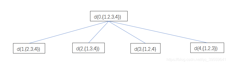
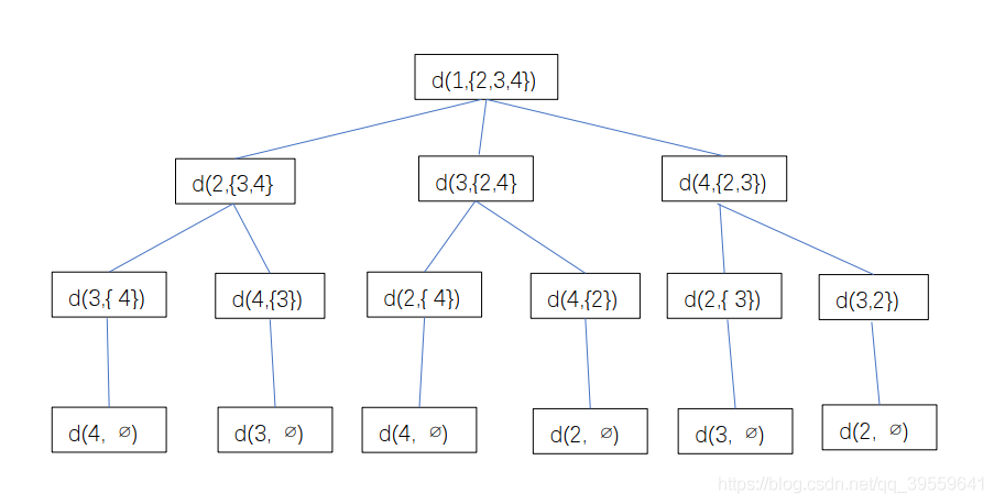
The recursive equation can be obtained as follows:

Now, we're going to find the optimal solution from the bottom up:

The bottom level will be:

The second last level will be:

The thrid last level will be:

Finally, we reach to the top level and got the optimal path:

In this algorithm, we take a subset 


Initially, all residences are unvisited, and the visit starts from the residence 
On the other hand, if the number of residences is greater than 
Finally, the algorithm returns the minimum distance as a TSP solution.
Here we use a dynamic approach to calculate the cost function 

In the dynamic algorithm for TSP, the number of possible subsets can be at most 


[1] Papadimitriou, C.H.; Steiglitz, K. (1998), Combinatorial optimization: algorithms and complexity, Mineola, NY: Dover, pp.308-309.
[2] Tucker, A. W. (1960), "On Directed Graphs and Integer Programs", IBM Mathematical research Project (Princeton University)
[3] Dantzig, George B. (1963), Linear Programming and Extensions, Princeton, NJ: PrincetonUP, pp. 545–7, ISBN 0-691-08000-3, sixth printing, 1974.
[4] Velednitsky, Mark (2017). "Short combinatorial proof that the DFJ polytope is contained in the MTZ polytope for the Asymmetric Traveling Salesman Problem". Operations Research Letters. 45 (4): 323–324. arXiv:1805.06997. doi:10.1016/j.orl.2017.04.010. S2CID 6941484.
[5] Bektaş, Tolga; Gouveia, Luis (2014). "Requiem for the Miller–Tucker–Zemlin subtour elimination constraints?". European Journal of Operational Research. 236 (3): 820–832. doi:10.1016/j.ejor.2013.07.038.