                                    ⠀⠀⠀⠀⠀⠀⠀⠀⠀⠀⠀⠀⠀⠀⠀⢀⣀⣤⣤⣴⣶⡆⠀⣶⣶⣦⣤⣤⣄⠀ ⢠⣾⣿⣦
                                    ⠀⠀⠀⠀⠀⠀⠀⠀⠀⠀⠀⣀⡀⢰⣿⣿⣿⣿⣿⣿⣿⡇⠀⣿⣿⣿⣿⣿⣿⡄⠘⢿⣿⠟
                                    ⠀⠀⠀⠀⠀⠀⠀⠀⢀⣴⣾⣿⣧⠀⢻⣿⣿⣿⣿⣿⣿⡇⠀⣿⣿⣿⣿⣿⣿⣿⠂⢠⣠⣤⣶⣦⡀
                                    ⠀⠀⠀⠀⠀⠀⣠⣾⣿⣿⣿⣿⣿⣇⠈⢿⣿⣿⣿⣿⣿⡇⠀⣿⣿⣿⣿⣿⣿⠏⢀⣿⣿⣿⣿⣿⣿⣦⡀
                                    ⠀⠀⠀⠀⠀⠘⢿⣿⣿⣿⣿⣿⣿⣿⡆⠘⣿⣿⣿⣿⣿⡇⠀⣿⣿⣿⣿⣿⡏⠀⣾⣿⣿⣿⣿⣿⣿⡿⠋⢀
                                    ⠀⠀⠀⣴⣿⣦⡀⠙⢿⣿⣿⣿⣿⣿⣿⡄⠸⣿⣿⣿⣿⡇⠀⣿⣿⣿⣿⡟⠀⣼⣿⣿⣿⣿⣿⣿⠟⢀⣴⣿⣧
                                    ⠀⠀⣼⣿⣿⣿⣿⣦⡀⠙⢿⣿⣿⣿⣿⣷⡀⢹⣿⣿⣿⡇⠀⣿⣿⣿⡿⠁⣰⣿⣿⣿⣿⣿⠟⢁⣴⣿⣿⣿⣿⣧
                                    ⠀⣼⣿⣿⣿⣿⣿⣿⣿⣦⡀⠙⢿⣿⣿⣿⣧⠀⢻⣿⣿⡇⠀⣿⣿⣿⠃⢰⣿⣿⣿⣿⠟⢁⣴⣿⣿⣿⣿⣿⣿⣿⣧
                                    ⠀⠛⠿⢿⣿⣿⣿⣿⣿⣿⣿⣦⡀⠙⢿⣿⣿⣇⠀⢿⣿⡇⠀⣿⣿⠇⢠⣿⣿⣿⠟⢁⣴⣿⣿⣿⣿⣿⣿⣿⣿⡿⠟⠃
                                    ⣼⣶⣤⣄⡈⠙⠛⠿⣿⣿⣿⣿⣿⣦⡀⠙⢿⣿⡆⠈⠛⠃⠀⠛⠋⠀⣾⣿⠟⠁⣠⣾⣿⣿⣿⣿⡿⠿⠛⠉⣀⣠⣴⣶⡄
                                    ⣿⣿⣿⣿⣿⣿⣶⣤⣀⡉⠙⠻⢿⣿⣿⣦⠀⠁⠀⠀⠀⠀⠀⠀⠀⠀⠈⠁⢠⣾⣿⣿⠿⠛⠋⢁⣠⣴⣶⣿⣿⣿⣿⣿⣿⡀
                                    ⢻⣿⣿⣿⣿⣿⣿⣿⣿⣿⣷⣦⣤⣀⠉⠃⠀⠀⠀⠀⠀⠀⠀⠀⠀⠀⠀⠀⠈⠋⢁⣀⣤⣶⣿⣿⣿⣿⣿⣿⣿⣿⣿⣿⣿⣧
                                    ⢸⣿⣿⣿⣿⣿⣿⣿⣿⣿⣿⣿⣿⣿⡏⠀⠀⠀⠀⠀⠀⠀⠀⠀⠀⠀⠀⠀⠀⠘⣿⣿⣿⣿⣿⣿⣿⣿⣿⣿⣿⣿⣿⣿⡟⠁⠀⣠⣶⣄
                                    ⠀⣤⣤⣤⣤⣤⣤⣤⣤⣤⣤⣤⣤⣤⡄⠀⠀⠀⠀⠀⠀⠀⠀⠀⠀⠀⠀⠀⠀⠀⣤⣤⣤⣤⣤⣤⣤⣤⣤⣤⣤⣤⣤⣤⡄⠀ ⢻⣿⣿⡿
                                    ⠀⠘⣿⣿⣿⣿⣿⣿⣿⣿⣿⣿⣿⠿⠓⠀⠀⠀⠀⠀⠀⠀⠀⠀⠀⠀⠀⠀⠀⣸⣿⣿⣿⣿⣿⣿⣿⣿⣿⣿⣿⣿⣿⣿⡿⠂⠀⠈⠙⠋
                                    ⠀⠀⠘⣿⣿⣿⣿⣿⠿⠛⠋⢁⣠⣤⣶⣧⠀⠀⠀⠀⠀⠀⠀⠀⠀⠀⠀⠀⢰⣿⣿⣿⣿⣿⣿⣿⣿⣿⣿⣿⣿⣿⠟⠋
                                    ⠀⠀⠀⠘⠟⠋⢉⣀⣤⣶⣿⣿⣿⣿⠟⠁⣠⣦⣄⡀⠀⠀⠀⠀⠀⠀⣤⣦⡈⠻⣿⣿⣿⣿⣿⣿⣿⣿⣿⡿⠛⠁
                                    ⠀⠀⠀⠀⠀⠘⢿⣿⣿⣿⣿⣿⠟⠁⣠⣾⣿⣿⣿⣿⣿⣶⣶⣾⣧⠀⢻⣿⣿⣦⡈⠻⣿⣿⣿⣿⡿⠟⠉
                                    ⠀⠀⠀⠀⠀⠀⠀⠙⠿⣿⡟⠁⣠⣾⣿⣿⣿⣿⣿⣿⣿⣿⣿⣿⣿⣇⠈⠿⢿⣿⣿⣦⡈⠻⠛⠉
                                    ⠀⠀⠀⠀⠀⠀⠀⠀⠀⠈⠀⠺⢿⣿⣿⣿⣿⣿⣿⣿⣿⣿⣿⣿⣿⠋⢀⣤⣤⡈⠙⠋⠁
                                    ⠀⠀⠀⠀⠀⠀⠀⠀⠀⠀⠀⠀⠀⠀⠉⠙⠛⠻⠿⠿⠿⠿⠿⠿⠇⠀ ⣿⣿⣿⡇
                                    ⠀⠀⠀⠀⠀⠀⠀⠀⠀⠀⠀⠀⠀⠀⠀⠀⠀⠀⠀⠀⠀⠀⠀⠀⠀⠀   ⠈⠙⠋

                         /██   /██   /██   /██   /██████    /██████     /██████    /██      /██   /███████
                        | ██  | ██  | ███ | ██  |_  ██_/   /██__  ██   /██__  ██  | ███    /███  | ██__  ██
                        | ██  | ██  | ████| ██    | ██    | ██  \__/  | ██  \ ██  | ████  /████  | ██  \ ██
                        | ██  | ██  | ██ ██ ██    | ██    | ██        | ████████  | ██ ██/██ ██  | ███████/
                        | ██  | ██  | ██  ████    | ██    | ██        | ██__  ██  | ██  ███| ██  | ██____/
                        | ██  | ██  | ██\  ███    | ██    | ██    ██  | ██  | ██  | ██\  █ | ██  | ██
                        |  ██████/  | ██ \  ██   /██████  |  ██████/  | ██  | ██  | ██ \/  | ██  | ██
                         \______/   |__/  \__/  |______/   \______/   |__/  |__/  |__/     |__/  |__/
Version: 1.0.1
Authors
Nathan Barros de Souza
Joyce Tavares Lopes
Luís Fernando Mercier Franco
This NVT-Monte Carlo algorithm was originally designed to test an equation of state developed for ellipsoidal molecules (Lopes and Franco, Ind. Eng. Chem. Res., 58, 16, 6850–6859, 2019). This thermodynamic model applies a perturbation theory, considering the reference fluid as hard ellipsoids of revolution interacting via short-range repulsive forces according to the Hard Gaussian Overlap (HGO) approach (Berne and Pechukas, J. Chem. Phys., 56, 4213, 1972) and the perturbed system ruled by attractive forces defined by a symmetrically spherical square-well potential. Our aim is to investigate the valid limits of reduced number density (κρ*) and ellipsoidal elongation (κ) by calculating the first- and second-order perturbation coefficients, as well as the orientational ordering parameter of a uniaxial nematic phase. Please check our paper for more details.
- 1. Disclaimer
- 2. Language
- 3. Building and Compilation
- 4. Reporting Errors
- 5. Data Input
- 6. Initial Configuration
- 7. Files and Folders
- 8. Running the Code
- 9. Citing Us
The authors make no warranties about the use of this software. The authors hold no liabilities for the use of this software. The authors do not recommend the use of this software whatsoever. The algorithm is made freely available to clarify any details discussed in the paper. All information contained herein regarding any specific methodology does not constitute or imply its endorsement or recommendation by the authors.
The main program, subroutines, modules, and functions contain some explanatory comments and are mainly written in Fortran 95. The user can look for more information on Fortran language here.
All programs, subroutines, modules, and functions must be compiled together due to their interdependence. For compilation, we have used GFortran, the GNU Fortran compiler, which is part of the GNU Compiler Collection (GCC). See more information on GFortran here. We tested the algorithm using two GFortran versions: a GCC version 9.3.0 in a Windows Subsystem for Linux (Ubuntu 20.04 LTS, Focal Fossa) and a GCC version 8.2.1 in a Red Hat Enterprise Linux OS. Visit the GCC Website for more information on these versions.
We have built the code using the following command line:
gfortran -O3 main.f95 functions.f95 subroutines.f95 module_folders.f95 module_global_variables.f95 module_initial_configuration.f95 module_variable_initialization.f95 -o main.out
The -O3 option is an optimization flag that improves compilation performance at the expense of compilation time. It includes all
optimization options from -O1 and -O2 flags. Check this link
for more details. In some cases, it might be necessary to add the -fno-range-check runtime option to disable range checking of input
values during integer READ operations. Click here
for more information.
If you spot an error in the program files and all other documentation, please submit an issue report using the Issues tab.
Before running the code, the user should first prepare an input file named mchgo_input.ini containing most of the external variables.
These variables are read by the module Variable Initialization.
An example of an input file was provided and explained below
(d0 means double precision):
number_of_particles= 500
reduced_temperature= 2.5d0
n_lambda= 4
lambda_values= 1.2d0 1.3d0 1.5d0 1.8d0
quaternion_angle= 0.d0
max_steps= 20000000
equilibration= 10000000
n_save= 1000
n_adjust= 200
max_trans= 0.3d0
max_rot= 0.1d0
min_blockav= 600
max_blockav= 1000
trajectory_inquiry= N
coefficient_inquiry= Y
production_inquiry= Y
The entry number_of_particles corresponds to the number of particles inside your simulation box. This must be a number with
an exact cube root, which depends on the selected configuration of the crystalline structure: ∛N for a simple cubic structure,
∛(N/2) for a body-centered cubic structure, and ∛(N/4) for a face-centered cubic structure, where N is
the number of particles.
The entry reduced_temperature corresponds to the reduced thermodynamic temperature T* of the system.
The entry n_lambda corresponds to the number of attractive range parameters λ. For instance, if the user wants to calculate the perturbed potential
for four different attractive range parameters (e.g. 1.2, 1.3, 1.5, and 1.8), then n_lambda must be equal to 4.
The entry lambda_values corresponds to the values of the attractive range parameters. If the user selected multiple λ in the previous entry, then all
corresponding λ values must be entered sequentially here, as shown in the example above. It does not necessarily have to be in ascending order.
The entry quaternion_angle corresponds to the rotation angle of the molecules in the initial configuration. It is usually set to 0, since all particles
are initially oriented along the z-axis (body-fixed axis).
The entry max_steps corresponds to the number of simulation cycles.
The entry equilibration corresponds to the number of equilibration cycles. Therefore, the number of production cycles will be max_steps − equilibration.
The entry n_save corresponds to the data saving frequency (inversely proportional relation). It means data will be written out in external files every
n_save cycles.
The entry n_adjust corresponds to the adjusment frequency of the maximum displacement (inversely proportional relation). It means the maximum displacement
(rotational and translational) will be adjusted every n_adjust cycles.
The entries max_trans and max_rot correspond to the initial values of the maximum translational displacement and maximum rotational displacement,
respectively.
The entries min_blockav and max_blockav correspond to minimum and maximum number of blocks used in the block-average subroutine, respectively. They
are necessary to estimate the statistical inefficiency.
The last three entries are inquiry variables. trajectory_inquiry inquires whether the molecular trajectory (position and orientation) is going to be written out in
external files. Type N for a negative answer or Y for an affirmative one. The trajectory file is properly formatted to be uploaded in OVITO, a scientific
visualization and analysis software for atomistic and particle simulation data. coefficient_inquiry inquires whether the block-average subroutine will be
called at the end of the Monte Carlo simulation to estimate averages and uncertainties of some relevant variables. Type N for a negative answer or Y for an
affirmative one. production_inquiry inquires whether only production-related results will be written out in external files. Type Y for only
production-related results or N to also include equilibration results.
Reduced number density κρ* and elongation κ must be provided by the user on the fly.
The user is allowed to select one of three crystalline structures for the initial molecular configuration at the beginning of the simulation. Structures are either stretched, narrowed, or pure cubic geometries depending on the ellipsoidal elongation. The available structures are: simple cube (SC), body-centered cube (BCC), or face-centered cube (FCC). Like κρ* and κ variables, the initial molecular configuration is also provided by the user on the fly.
The initial configuration (position and orientation of particles) is, by default, written out in an external file and is also properly formatted to be uploaded in OVITO. An example of these crystalline structures can be seen below for κρ* = 0.5.
Figure 01-A. Example of a simple cubic structure. Particles are hard spheres (κ = 1). Number of particles: 512.
Click here to zoom the figure in.
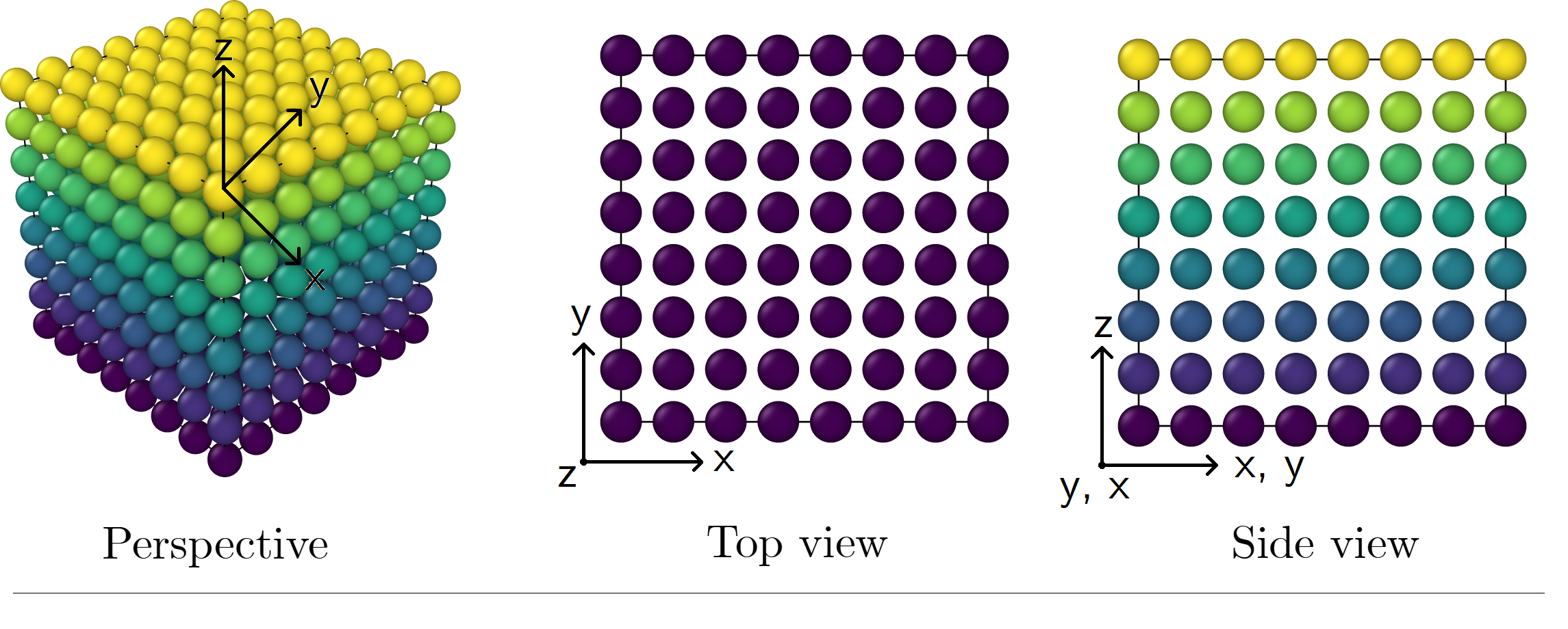
Figure 01-B. Example of a narrowed body-centered cubic structure. Particles are oblate ellipsoids of revolution (κ < 1.0).
Number of particles: 686. Click here to zoom the figure in.
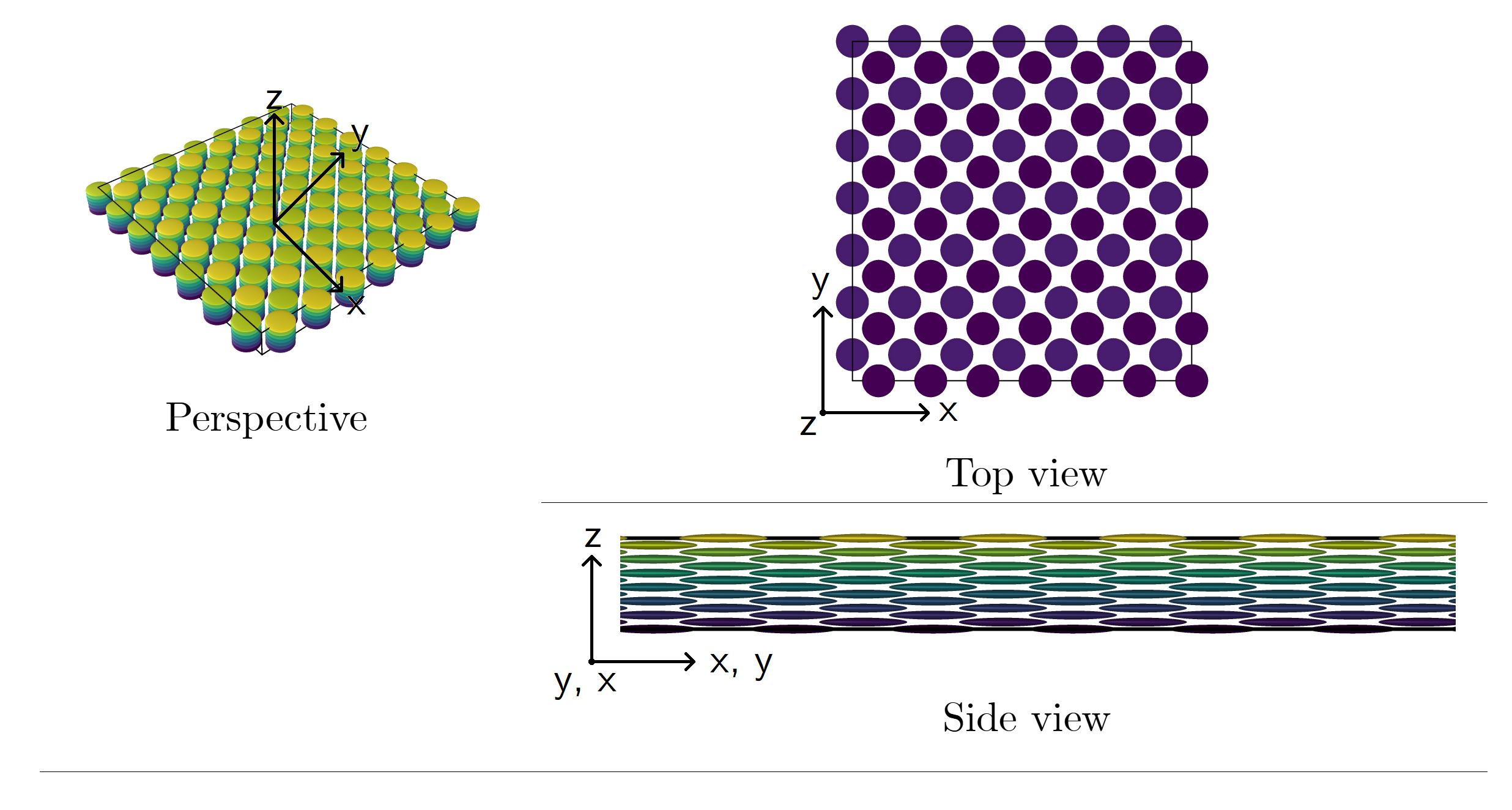
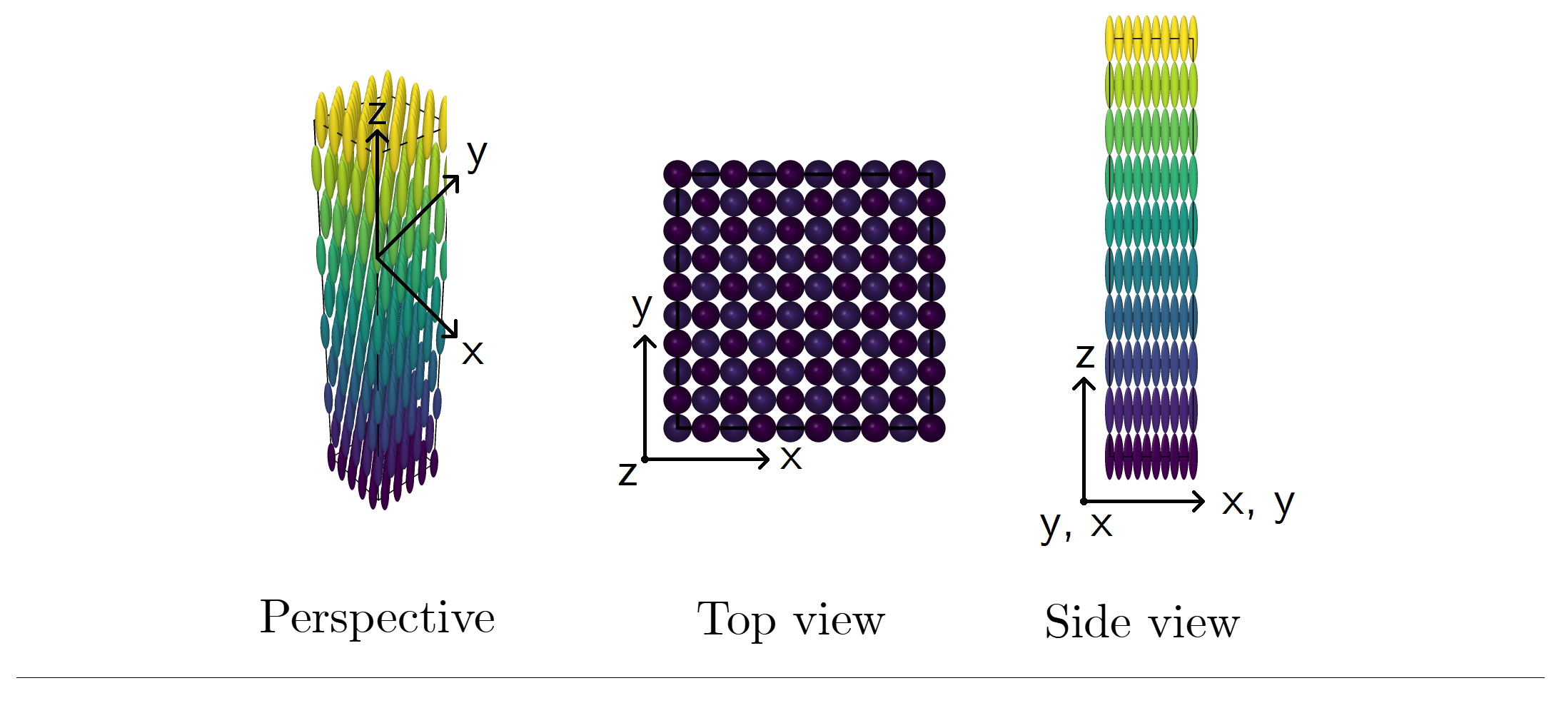
Figure 01-C. Example of a stretched face-centered cubic structure. Particles are prolate ellipsoids of revolution (κ > 1.0).
Number of particles: 500. Click here to zoom the figure in.
NOTE: Please pay attention to choose an initial configuration that matches the valid number of particles for that structure.
After choosing the crystalline structure and inserting the values of κρ* and κ, the program will organize the output files and directories.
The program creates 6 parent directories in total. To better organize the output files, all directories (or subdirectories) contains a date folder, corresponding to the
starting date of the simulation (e.g. 20210101 means the simulation strated at January 1st, 2021).
The Initial_Configuration/ directory and OVITO/ subdirectory store the initial configuration file, consisting of position and orientation of
particles, as well as the molecular geometry.
The Trajectories/ directory stores the trajectory file, consisting of the same properties of the initial configuration file. These properties are written out every
n_save cycles.
NOTE: the algorithm creates this directory regardless the users' choice to write out the respective file.
The Potential/ directory stores the potential energy of the perturbed system. This property is written out every n_save cycles.
The algorithm also creates one attractive range subfolder for every selected λ. The calculated potential energy is then stored on each respective
subfolder.
The Ratio/ directory stores information on equilibration cycles (acceptance ratio, maximum displacement, and ratio threshold). This information is separated into
two subfolders: Rotation/ for rotational movements and Translation/ for translational movements.
The Order_Parameter/ directory stores the nematic order parameter. This property is written out every n_save cycles.
The Perturbed_Coefficient/ directory stores the results generated by the block-average subroutine. Since these results are based on the potential energy of the perturbed system, they are also separated in subfolders based on the attractive range parameter.
NOTE: the algorithm creates this directory regardless the users' choice to call the respective subroutine.
The aforementioned folders are created by executing a shell command via an intrinsic function called SYSTEM. Please note that which shell is used to invoke the
command line is system-dependent and environment-dependent. Check this link for more information.
File names are based on the information they hold, followed by the reduced number density and elongation parameters that were used to create them. Files with identical names
are always overwritten. Thus, running simulations with the same κρ* and κ at the same date will always overwrite existing data.
Because shell commands are executed during simulation and files are opened and written, we recommend Linux's users to run the compiled code with the sudo command
below to avoid administrative issues.
sudo ./main.out
After setting up the molecular structure and organizing folders and files, the algorithm will print out a user-friendly simulation summary. Here the user will be able to
review all important parameters (number of cycles, attractive range, reduced variables etc.) prior to the Monte Carlo simulation itself. After checking everything up, the
user must press a KEY to continue the simulation.
The first simulation goal is to determine any possible molecular overlaps in the initial configuration. The overlap check is made by calculating the contact distance according to the Hard Gaussian Overlap (HGO) model (Berne and Pechukas, J. Chem. Phys., 56, 4213, 1972). An overlap is detected when the HGO contact distance is greater than or equal to the distance between the centers of mass of two molecular ellipsoids of revolution. If that happens, the simulation is immediately interrupted. Otherwise, it proceeds to the Metropolis sampling algorithm (Metropolis et al., J. Chem. Phys., 21, 1087, 1953).
During a sampling cycle, a particle is randomly selected according to a linear congruential generator (LCG). The LCG is a pseudorandom number generator that yields a sequence of randomized numbers from the uniform distribution over the range 0 ≤ x < 1. Afterwards, a trial move is performed for the selected particle. Trial moves are divided into two equiprobable events: a translational and a rotational displacement. Only one kind of molecular displacement can take place at a time in each cycle. If the translational event is chosen, the selected particle will be randomly translated across the simulation box, limited to a maximum translational displacement (MTD). On the other hand, if the rotational event is chosen, the selected particle will be randomly rotated around its center of mass, limited to a maximum rotational displacement (MRD). Rotations are implemented via quaternions algebra. Read pages 106-111 of Allen and Tildesley (Computer Simulation of Liquids, 2nd edition, 2017) for more details.
After randomly displacing a particle, the algorithm proceeds to the Metropolis' criterion, which can be simplified to a single molecular overlap check in the case of hard-core geometries. Thus, the trial move is inspected to check any possible overlapping configurations. If overlap is detected, the trial move is immediately rejected and a new cycle begins. Otherwise, the trial move is accepted and the system is updated in terms of position and orientation of the selected particle and potential energy. This energy is computed in accordance with the square-well (SW) potential.
The simulation is splitted into two phases: the equilibration phase and the production phase. During equilibration phase, the maximum displacements (MD) are either positively or
negatively adjusted by 5% of their current value. If the number of accepted moves divided by the
number of trial moves (acceptance ratio) is higher than a initially fixed threshold of 0.5, then the MDs are positively adjusted, and vice-versa. In some cases, the
equilibration phase
performs poorly. For instance, for low density systems composed of quasi-spherical particles (i.e.
κ = 0.9), most of the trial moves are accepted regarding rotational displacements. In that case, the sampling generally fails to generate overlapping
configurations and thus the MRD will frequently undergo a positive adjustment. Eventually, the MRD skyrockets to impracticable values, leading to mathematical inaccuracies.
Therefore, we decided to replace the fixed threshold by a "dynamic threshold". This dynamic threshold is arbitrarily modified everytime the MD values reach a limit. For MTD,
the upper limit is the maximum length of the simulation box, while the lower limit is 1 ⨯ 10⁻⁵. For MRD, the upper limit is π
(half-turn
condition), while the lower limit is 2 ⨯ 10⁻⁴ / L, where L is the largest ellipsoidal axis diameter. Except for the upper limit of the
MRD, the other limits are merely arbitrary. Hence, when the MDs reach the upper limit, the dynamic threshold increases, and when the MDs reach the lower limit, the dynamic
threshold decreases.
NOTE: Whenever the ratio threshold is modified, the simulation is reset to its initial values (configuration, energy, etc.), except for the current equilibration
cycle. It is noteworthy to mention that we did not implement a simulation reset in our paper (the final results are not significantly different).
During production phase, the potential energy of the perturbed system is computed and the nematic order parameter is calculated. The latter is calculated via a tensor diagonalization method (Zannoni, 1979. In: Luckhurst and Gray (eds.), The Molecular Physics of Liquid Crystals, 1979, pp. 51–83).
After completing the Metropolis sampling, the algorithm evokes the block-average subroutine (depending on the user's choice). Read pages 281-287 of Allen and Tildesley (Computer Simulation of Liquids, 2nd edition, 2017) for more details. This subroutine estimates the averages and uncertainties of the first- and second-order perturbation coefficients, as well as the total Helmholtz free energy of the perturbed system. In the case of the Helmholtz free energy, due to high exponential terms that leads to computational inaccuracies in some machine's architectures, we applied a mathematical relation to replace an exponential sum by a more practicable expression, saving processing time and avoiding overflow errors. Check this Supplementary Material (Abreu and Escobedo, J. Chem. Phys., 124, 054116, 2006) for more information.
At the end of the simulation, the program writes out a log file containing all simulation details. Later simulations will only append information to the log file instead of overwriting it.
If our code was useful in any way, we kindly ask you to cite our work "Thermodynamic perturbation theory coefficients for ellipsoidal molecules".
“With thermodynamics, one can calculate almost everything crudely; with kinetic theory, one can calculate fewer things, but more accurately; and with statistical mechanics, one can calculate almost nothing exactly.” -- Eugene P. Wigner