Tutorial
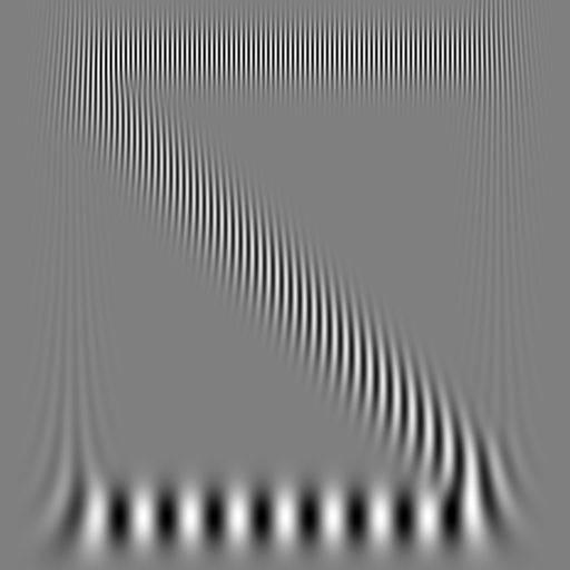
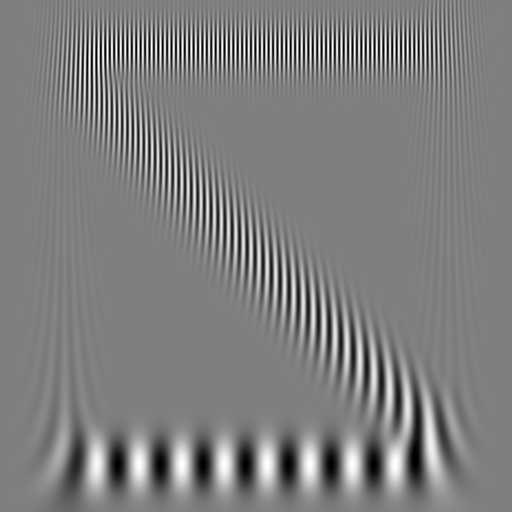
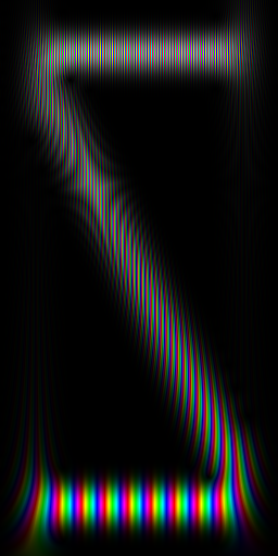
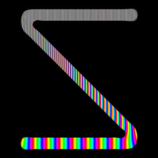
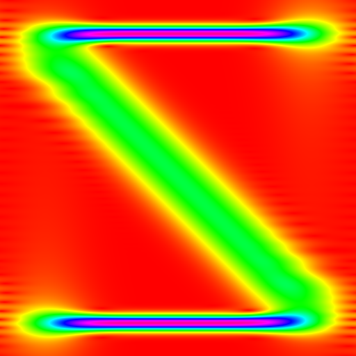
What you see here is a spectrogram with X-axis linear time and Y-axis linear frequency scales. It shows three waves: A constant low frequency, a constant high frequency and one with a frequency that falls linearly.


The following color schemes are supported:
- REAL_GRAYSCALE: Only the real part is shown.
- IMAGINARY_GRAYSCALE: Only the imaginary part is shown.
- AMPLITUDE_GRAYSCALE: Only the amplitude is shown.
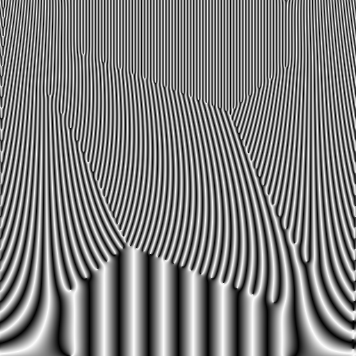
- PHASE_GRAYSCALE: Only the phase is shown.
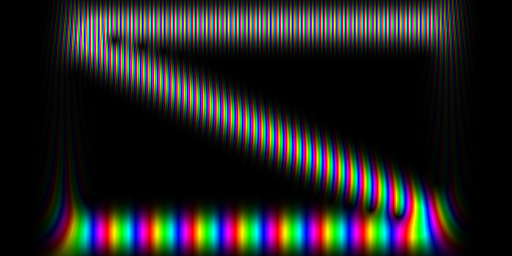
- EQUIPOTENTIAL: Only the amplitude is shown and mapped to the physical energy level of different colors. So red is low, green is in the middle and blue is high.
- RAINBOW_WALLPAPER: Phase is modeled as the colors hue and the amplitude is the colors brightness.


The following synchrosqueeze modes are supported:
- IDENTITY: Deactivates synchrosqueeze
- DERIVATIVE_QUOTIENT: Intermediate output of synchrosqueeze
- SOBEL: Activates synchrosqueeze with a sobel edge filter
- NEAREST_SAMPLE: Activates synchrosqueeze with nearest sampling filter
- LINEAR_SAMPLE: Activates synchrosqueeze with linear sampling filter
import ccwt, numpy, math

height = 512
width = 512
border = 64
enable_complex = True

def generate_wave(frequency_range, frequency_offset):
    phases = numpy.zeros(width)
    for t in range(0, width):
        phases[t] = (frequency_range*t/width+frequency_offset)*(math.pi*2.0*t/width)
    if enable_complex:
        wave = numpy.exp(phases*1.j)
    else:
        wave = numpy.cos(phases)
    for t in range(0, width):
        wave[t] *= (t > border) and (t < width-border)
    return wave

frequency_range = height*0.25
frequency_band = ccwt.frequency_band(height, frequency_range)
signal = generate_wave(-0.5*frequency_range, frequency_range)+generate_wave(0.0, 0.09375*frequency_range)+generate_wave(0.0, (1.0-0.09375)*frequency_range)
fourier_transformed_signal = ccwt.fft(signal)

for synchrosqueeze_mode in range(0, 4):
    for color_scheme in range(0, 6):
        with open("{}_{}.png".format(synchrosqueeze_mode, color_scheme), "w") as outfile:
ccwt.render_png(outfile, synchrosqueeze_mode, color_scheme, 0.0, fourier_transformed_signal, frequency_band, width)If you would downsample the input you would loose the high frequencies and if you would downsample the output you would waste lots of computational power. But this library supports downsampling in the middle of the process and lets you keep high frequencies while saving computational power.
frequency_band = ccwt.frequency_band(int(height/2), frequency_range)
with open('size_h.png', 'w') as outfile:
    ccwt.render_png(outfile, ccwt.IDENTITY, ccwt.RAINBOW_WALLPAPER, 0.0, fourier_transformed_signal, frequency_band, width)
frequency_band = ccwt.frequency_band(height, frequency_range)
with open('size_w.png', 'w') as outfile:
ccwt.render_png(outfile, ccwt.IDENTITY, ccwt.RAINBOW_WALLPAPER, 0.0, fourier_transformed_signal, frequency_band, int(width/2))Logarithmic intensity rendering can sharpen the edges.

And also be used to invert the result.
fourier_transformed_signal = ccwt.fft(signal*2.0)
with open('logarithmic_intensity_m.png', 'w') as outfile:
    ccwt.render_png(outfile, ccwt.IDENTITY, ccwt.RAINBOW_WALLPAPER, 1.2, fourier_transformed_signal, frequency_band, width)
fourier_transformed_signal = ccwt.fft(signal*2.0)
with open('logarithmic_intensity_l.png', 'w') as outfile:
ccwt.render_png(outfile, ccwt.IDENTITY, ccwt.RAINBOW_WALLPAPER, 1.0/1.2, fourier_transformed_signal, frequency_band, width)Because we are using fft to accelerate the convolutions both ends of a signal are connected and influence each other.


The easiest way to get rid of this effect is by adding some padding zeros in the input signal. This library can take care of adjusting all other parameters accordingly as well.
border = 0
signal = generate_wave(frequency_range*0.5, 0.0)
fourier_transformed_signal = ccwt.fft(signal)
with open('padding_0.png', 'w') as outfile:
    ccwt.render_png(outfile, ccwt.IDENTITY, ccwt.EQUIPOTENTIAL, 0.0, fourier_transformed_signal, frequency_band, width)

padding = 32
fourier_transformed_signal = ccwt.fft(signal, padding)
with open('padding_1.png', 'w') as outfile:
ccwt.render_png(outfile, ccwt.IDENTITY, ccwt.EQUIPOTENTIAL, 0.0, fourier_transformed_signal, frequency_band, width, padding)Values near zero have better frequency resolution, values towards infinity have better time resolution.

frequency_band = ccwt.frequency_band(height, frequency_range, 0.0, 0.0, 1.0/5.0)
with open('deviation_l.png', 'w') as outfile:
    ccwt.render_png(outfile, ccwt.IDENTITY, ccwt.EQUIPOTENTIAL, 0.0, fourier_transformed_signal, frequency_band, width)
frequency_band = ccwt.frequency_band(height, frequency_range, 0.0, 0.0, 1.0*5.0)
with open('deviation_h.png', 'w') as outfile:
ccwt.render_png(outfile, ccwt.IDENTITY, ccwt.EQUIPOTENTIAL, 0.0, fourier_transformed_signal, frequency_band, width)When analyzing music we often want exponential frequency bands instead of linear ones like this:
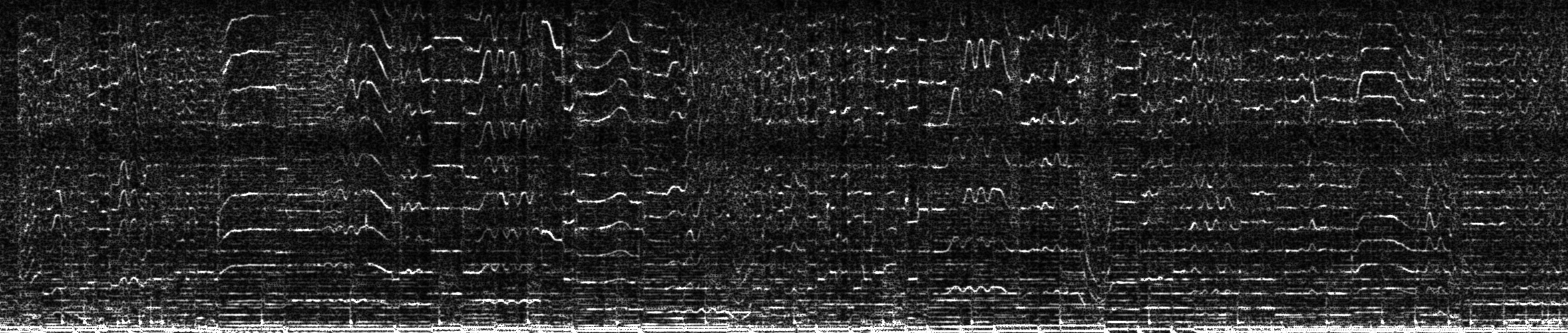
But just stretching the image leads to visible distortion because the same deviation is applied to all frequencies.
Luckily this library can take care of that and automatically adjust the deviation over the frequencies.
You can even specify your own frequency band, which is composed of an 2D array with 2 columns and n rows. The first column are the frequencies and the second their derivative (which can also be gained numerically).
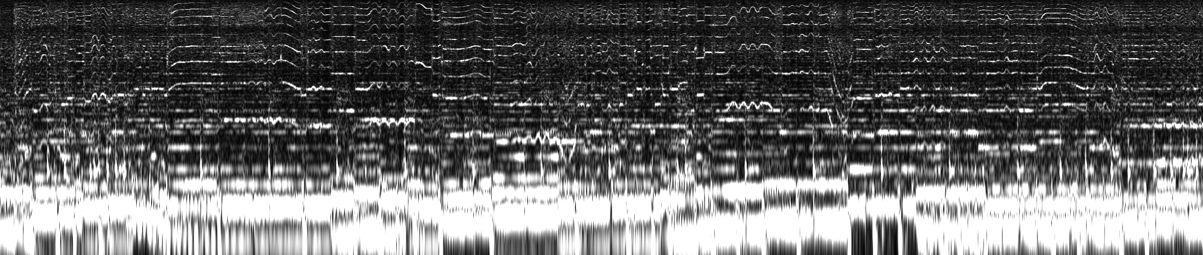
import ccwt, numpy, math, librosa
audio_file = librosa.load('music.ogg')
signal = audio_file[0]*10.0 # Input scale factor (to be adjusted)
samples_per_second = audio_file[1]
length_in_seconds = float(len(signal))/samples_per_second
pixels_per_second = 100
height = 500
# These frequencies are measured in Hz so we multiply them with length_in_seconds to get the frequencies over the entire signals length
minimum_frequency = 44.0*length_in_seconds
maximum_frequency = 5200.0*length_in_seconds
frequency_band = ccwt.frequency_band(height, maximum_frequency-minimum_frequency, minimum_frequency) # Linear
with open('frequency_band_0.png', 'w') as outfile:
ccwt.render_png(outfile, ccwt.IDENTITY, ccwt.AMPLITUDE_GRAYSCALE, 0.0, ccwt.fft(signal), frequency_band, int(length_in_seconds*pixels_per_second))
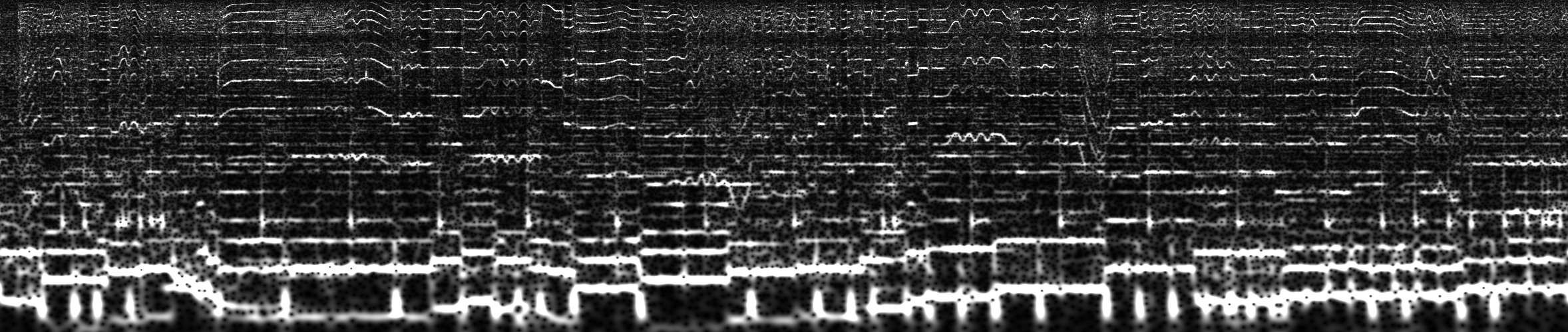
frequency_base = 2.0 # Each octave doubles the frequency
minimum_octave = math.log(minimum_frequency)/math.log(frequency_base)
maximum_octave = math.log(maximum_frequency)/math.log(frequency_base)
frequency_band = ccwt.frequency_band(height, maximum_octave-minimum_octave, minimum_octave, frequency_base) # Exponential
with open('frequency_band_2.png', 'w') as outfile:
ccwt.render_png(outfile, ccwt.IDENTITY, ccwt.AMPLITUDE_GRAYSCALE, 0.0, ccwt.fft(signal), frequency_band, int(length_in_seconds*pixels_per_second))The fft calculation can account for a big part of the computation time needed and is not affected by most parameters (except for the length of the input obviously and the padding). Thus it is a good idea to reuse it and even storing it to disk if you want to analyze it multiple times with varying parameters on different occasions.
The fft of a real signal produces a half as long but complex result. Therefore the second half of the result is 0 and this can be used to save memory when storing the fft result.
fourier_transformed_signal = fourier_transformed_signal[:len(fourier_transformed_signal)/2+1]
save_to_file(fourier_transformed_signal)

fourier_transformed_signal = load_from_file()
fourier_transformed_signal = numpy.concatenate((fourier_transformed_signal, numpy.zeros(len(fourier_transformed_signal)-2)))If you want to process the result programmatically you can just skip the first three parameters of render_png and use numeric_output instead.
result = ccwt.numeric_output(frequency_band, fourier_transformed_signal, width, padding, thread_count)The methods fft, render_png and numeric_output all support multithreading by adding a thread_count as last parameter. Keep in mind:
- It should only be used on large amounts of data else it might even slowdown the process.
- The maximum number of threads which can benefit you is the number of physical cores on your machine.
- It may vary over different calls and doesn't need to be the same in a fft call and subsequent render_png or numeric_output calls.
- Default value is 1 (no multithreading), 2 means one additional thread being spawned and so on.
fourier_transformed_signal = ccwt.fft(signal, padding, thread_count)
with open('out.png', 'w') as outfile:
    ccwt.render_png(outfile, ccwt.IDENTITY, ccwt.AMPLITUDE_GRAYSCALE, 0.0, fourier_transformed_signal, frequency_band, width, padding, thread_count)
ccwt.numeric_output(fourier_transformed_signal, frequency_band, width, padding, thread_count)