Stochastic gradient descent (SGD) in contrast performs a parameter update for each training example x(i) and label y(i):θ=θ−η⋅∇θJ(θ;x(i);y(i)).
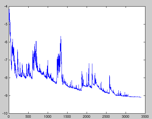
Batch gradient descent performs redundant computations for large datasets, as it recomputes gradients for similar examples before each parameter update. SGD does away with this redundancy by performing one update at a time. It is therefore usually much faster and can also be used to learn online. SGD performs frequent updates with a high variance that cause the objective function to fluctuate heavily as in Image 1.
While batch gradient descent converges to the minimum of the basin the parameters are placed in, SGD's fluctuation, on the one hand, enables it to jump to new and potentially better local minima. On the other hand, this ultimately complicates convergence to the exact minimum, as SGD will keep overshooting. However, it has been shown that when we slowly decrease the learning rate, SGD shows the same convergence behaviour as batch gradient descent, almost certainly converging to a local or the global minimum for non-convex and convex optimization respectively. Its code fragment simply adds a loop over the training examples and evaluates the gradient w.r.t. each example. Note that we shuffle the training data at every epoch as explained in this section.
for i in range(nb_epochs):
  np.random.shuffle(data)
  for example in data:
    params_grad = evaluate_gradient(loss_function, example, params)
    params = params - learning_rate * params_grad
MIT