perceptual-kalman-filters

Implementation of demo from "PKF: online state estimation under a perfect perceptual quality constraint" (Freirich et al., 2023) (Arxiv: https://arxiv.org/abs/2306.02400) (Poster: https://neurips.cc/media/PosterPDFs/NeurIPS%202023/71479.png?t=1699544143.6985004)

to execute run:

python ./run_osc_demo.py

or

./run_demo.sh

Citing us:

If you find our work inspiring, please cite us using the following Bibtex entry:

 @article{freirich2023perceptual,
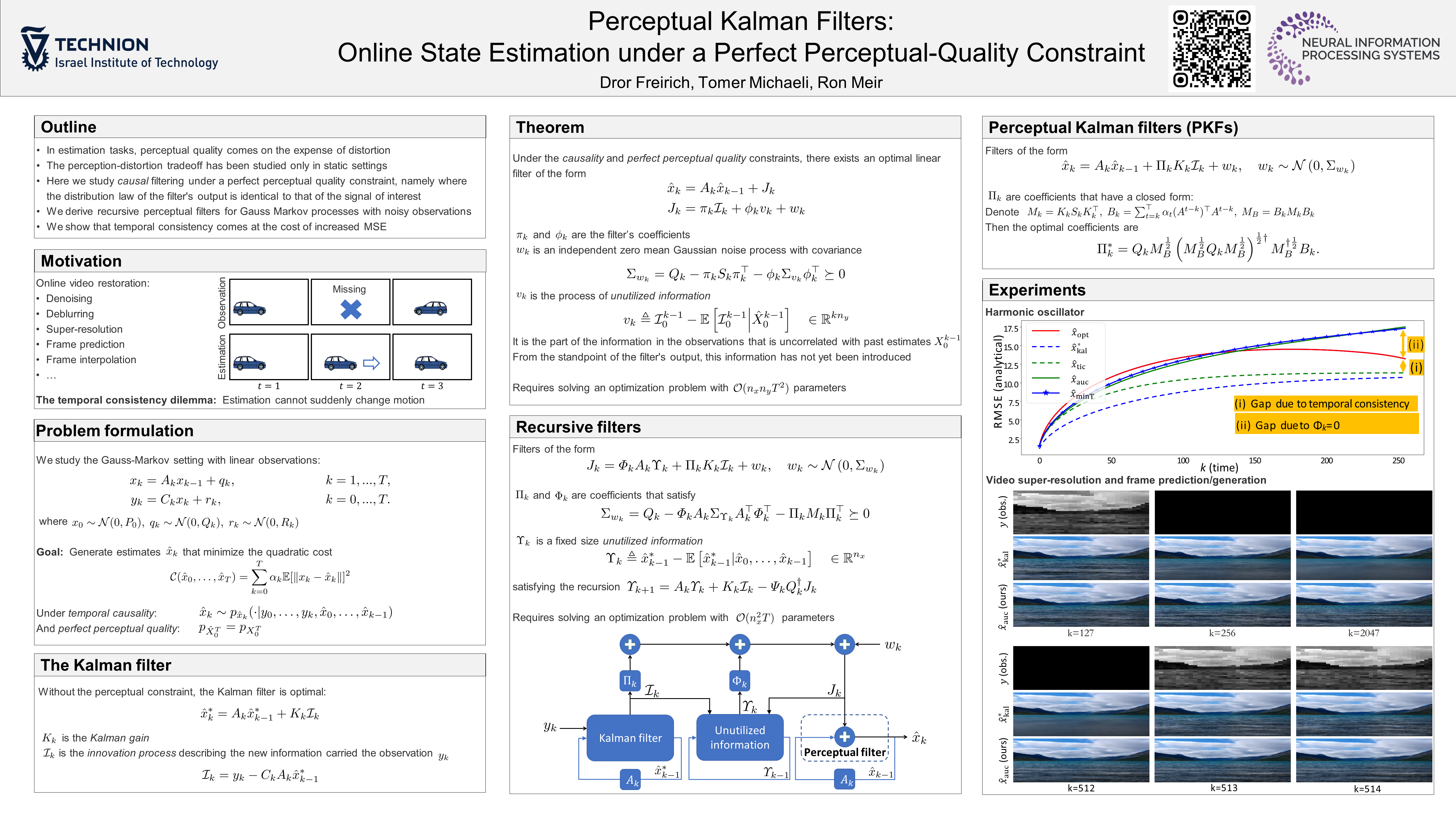
  title={Perceptual Kalman Filters: Online State Estimation under a Perfect Perceptual-Quality Constraint},
  author={Freirich, Dror and Michaeli, Tomer and Meir, Ron},
  journal={arXiv preprint arXiv:2306.02400},
  year={2023}
  }

Motivation for perceptual filtering

Example: real time video streaming

Sensory data from the scene might be compressed/corrupted/missing.

Reconstruction to the viewer must be done in real-time.

reconstructed scene must look natural.

The latter demand for realism means that not only each frame should look as a natural image, but motion should look natural too. That makes us face the Temporal Consistency dilemma: Estimation cannot suddenly change the motion in the output video, because such an abrupt change would deviate from natural video statistics. Thus, although the method is aware of its mistake, it may have to stick to its past decisions.

What's in the paper?

We study the theoretic Gauss-Markov setting with linear observations:

$x_{k}=A_{k}x_{k-1}+q_{k}, k=1,...,T$,

$y_{k}=C_{k}x_{k}+r_{k}, k=0,...,T$.

$x_0,q_k,r_k$ are zero-mean Gaussian r.v.'s with covariance matrices $P_0,Q_k,R_k$.

The problem is to minimize the Quadratic cost under the Temporal causality and Perfect perceptual quality constraints:.

$$\mathcal C (\hat{x}_{0},\ldots,\hat{x}_{T}) = \sum_{k=0}^{T}\alpha_{k}E{\|{x}_{k}-\hat{x}_{k}\|^{2}}$$ $$\hat{x}_{k}\sim p_{\hat{x}_{k}}(\cdot|y_{0},\ldots,y_{k},\hat{x}_{0},\ldots,\hat{x}_{k-1})$$ $$p_{\hat{X}_{0}^{T}}=p_{X_{0}^{T}}$$

Without the perceptual constraint, the Kalman state is a MSE-optimal causal estimator.

$$\hat{x}^*_k = A_k \hat{x}^*_{k-1} + K_k \mathcal{I}_k$$

$K_k$ is the Kalman gain and the innovation process describes the new information carried by the observation $y_k$.

$$\mathcal{I}_k=y_{k}-C_{k}\hat{x}^*_{k|k-1}$$

We present the following formalism for linear perceptual filters with coefficients $\Pi_{k},\varPhi_{k}$

$$\hat{x}_{k}=A_{k}\hat{x}_{k-1}+J_k$$ $$J_{k}=\varPhi_{k}A_{k}\Upsilon_{k}+\Pi_{k}K_{k}\mathcal{I}_{k}+w_{k},\quad w_{k}\sim\mathcal{N}\left(0,\Sigma_{w_{k}}\right)$$ $$\Sigma_{w_{k}}=Q_{k}-\varPhi_{k}A_{k}\Sigma_{\Upsilon_{k}}A_{k}^{\top}\varPhi_{k}^{\top}-\Pi_{k}M_{k}\Pi_{k}^{\top}\succeq0$$

$\Upsilon_{k}$ is the unutilized information state

$$\Upsilon_{k}\triangleq\hat{x}_{k-1}^{*}-\mathbb{{E}}\left[\hat{x}_{k-1}^{*}|\hat{x}_{0},\ldots,\hat{x}_{k-1}\right]$$

given by the recursion

$$\varUpsilon_{k+1} = A_k\varUpsilon_{k} +K_k \mathcal{I}_k - \varPsi_k Q_k^\dagger J_k,$$ $$\Sigma_{\varUpsilon_{k+1}} = A_k \Sigma_{\varUpsilon_k} A_k^\top +M_k -\varPsi_k Q_k^\dagger \varPsi_k^\top,$$ $$\varPsi_k = M_k \Pi_k^\top +A_k \Sigma_{\varUpsilon_k} A_k^\top \varPhi_k^\top.$$

The Perceptual Kalman Filter (PKF)

We suggest the simplified form

$$J_{k}=\Pi_{k}K_{k}\mathcal{I}_{k}+w_{k},\quad w_{k}\sim\mathcal{N}\left(0,\Sigma_{w_{k}}\right)$$

Now, the optimal coefficients are given explicitly (see full details in our paper)

$$\Pi_{k}^* = Q_{k}M_{B}^{1/2}\left(M_{B}^{1/2}Q_{k}M_{B}^{1/2}\right)^{1/2 \dagger}M_{B}^{\dagger 1/2}B_{k}M_{k}M_{k}^{\dagger}$$

Algorithm - Perceptual Kalman Filter (PKF):

FOR k=1 to T DO:

calculate:

$$M_{k}=K_{k}S_{k}K_{k}^{\top}, B_{k}= \sum_{t=k}^{T} \alpha_{t}(A^{t-k})^{\top}A^{t-k}, M_{B}=B_{k}M_{k}B_{k}.$$

compute optimal gain:

$$\Pi_{k} = Q_{k}M_{B}^{1/2}\left(M_{B}^{1/2}Q_{k}M_{B}^{1/2}\right)^{1/2 \dagger}M_{B}^{\dagger 1/2}B_{k}M_{k}M_{k}^{\dagger}$$

sample:

$$w_{k}\sim \mathcal{N}\left(0,Q_{k}-\Pi_{k}M_{k}\Pi_{k}^{\top}\right).$$

update state:

$$\hat{x}_{k} = A\hat{x}_{k-1} + \Pi_{k}K_{k}\mathcal{I}_{k} + w_{k}$$

Visual demo

Watch the video: