Ex2.rst

Example 2: (Fine-Grained) Permutation Entropy

Import the x, y, and z components of the Lorenz system of equations.

Data = ExampleData('lorenz');

figure('Color', 'k')
plot3(Data(:,1), Data(:,2), Data(:,3), 'g.')
xlabel('x-component','color','g'),
ylabel('y-component','color','g'),
zlabel('z-component','color','g'),
view(-10,10), set(gca,'color','k'), axis square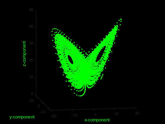

Calculate fine-grained permutation entropy of the z component in dits (logarithm base 10) with an embedding dimension of 3, time delay of 2, an alpha parameter of 1.234. Return Pnorm normalised w.r.t the number of all possible permutations (m!) and the condition permutation entropy (cPE) estimate.

Z = Data(:,3);

[Perm, Pnorm, cPE] = PermEn(Z, 'm', 3, 'tau', 2, 'Typex', 'finegrain', 'tpx', 1.234, 'Logx', 10, 'Norm', false)

>>> Perm = 1×3
    0   0.8687 0.9468

    Pnorm = 1×3
    NaN 0.8687 0.4734

    cPE = 1×2
    0.8687 0.0781