VAE and GAN

Content

1. Implementation of a VAE
2. Comparison of a GAN trained with Squared Hellinger distance vs Wasserstein distance
3. Implementation of a WGAN
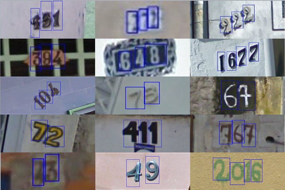
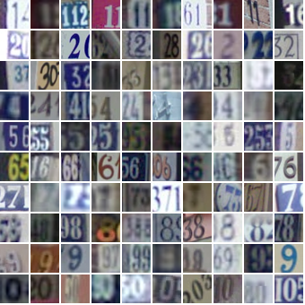
4. Training of the WGAN on Street View House Numbers

Bonus theoretical content touching:

• Autoregressive models
• Reparameterization trick
• Variational autoencoders (VAE)
• Normalizing flows
• Generative adversarial networks (GANs)

VAE

Variational Autoencoders (VAEs) are probabilistic generative models to model data distribution p(x). In this section, a VAE is trained on the Binarised MNIST dataset, using the negative ELBO loss. Note that each pixel in this image dataset is binary: The pixel is either black or white, which means each datapoint (image) is a collection of binary values. The likelihood p_θ(x|z), i.e. the decoder, is modelized as a product of bernoulli distributions.

GAN's Comparison

Generative Adversarial Network (GAN) enables the estimation of distributional measure between arbitrary empirical distributions. This Section implements a function to estimate the Squared Hellinger as well as one to estimate the Earth mover distance. This allows to look at and contrast some properties of the f-divergence and the Earth-Mover distance (Wasserstein GAN).

squared hellinger

Wasserstein

Comparison

WGAN

Train a generator to generate a distribution of images of size 32x32x3, namely the Street View House Numbers dataset (SVHN). The SVHN dataset can be downloaded here. The prior distribution considered is the isotropic gaussian distribution (p(z) = N(0, I)).

Street View House Numbers

Datasets' origin

Training set

Images generated by WGAN

Exploration of the latent space

We look if the model has learned a disentangled representation in the latent space. A random z is sampled from the prior distribution. Some small perturbations are added to the sample z for each dimension (e.g. for a dimension i, z_i = z_i + \epsilon). The samples are perturbed with 10 progressivily increasing values of \epsilon in (-5, -4, -3, -2, -1, 0, 1, 2, 3, 4) where \epsilon = 0 is the original sample.

Using a sample showing a 9, we see at Figure 3 that the perturbation can transform the 9 into a 'R', 2, 3, and a 8.

Similarly, a sample showing 2 can be turned into a 3 or 8

and the reverse is possible where a sample showing 3 can be transformed to a 2.

Finally, an interesting transformation found was that the perturbation could affect the thickness of the number.

Interpolating in the data space vs in the latent space

The difference between both interpolations is that (b) is only overlapping two images and gradually changing their transparency. It does not show intermediate images between z_0 and z_1. It fades z_0 into z_1 without changing the shapes contained. (a) uses the generator to create intermediary images between z_0 and z_1. It gradually generates images closer to z_1 in the latent space and farther to z_0. It is closer to showing how z_0 can morph into z_1.