Value-at-Risk-VaR-Modeling-in-Python

ARMA-GARCH Modeling, Volatility and Value at Risk (VaR) Forecasting in Python

Download Data from Yahoo Finance

import yfinance as yf
from yahoofinancials import YahooFinancials
start_date='2010-01-01'
end_date=end='2021-09-01'

sp_data= yf.download('SPY',  # List of tickers
                      start='2010-01-01', 
                      end='2021-09-01', 
                      progress=False)

ARIMA modeling

Box-Jenkins Methodology

Box-Jenkins approach applies ARIMA models to find the best fit of a univariate time series model that represent the stochastic process. This method is including a three steps modelling:

1. Identification: Based on the Autocorelation Function (ACF) and Partial Autocorrelation Function (PACF) it is possible to determine p, and q order of the ARIMA model. Also, we can use the Akaike Information Criterion (AIC) to identify the ARIMA order.
2. Estimation: Estimation of best ARMA(p,q) order.
3. Diagnostic checking: The ARMA process is valid when the residuals (ACF and PACF plots) are uncorrelated.

GARCH Modeling and Volatility

In order to model volatility, we use the Autoregressive Conditional Heteroscedasticity (ARCH) model. ARCH is a statistical model for time series data that describes the variance of the current error term as a function of the previous time periods’ error terms. The next step is to define the second part of the error term decomposition which is the conditional variance. For this purpose, we can use a GARCH(1, 1) models.

# GARCH normal model 
garch_norm= arch_model(sp_data['Log_Return'], p = 1, q = 1,
                      mean = 'constant', vol = 'GARCH', dist = 'normal')
# Fit the model
garch_norm_result = garch_norm.fit(update_freq = 4)

# Get summary
print(garch_norm_result.summary())

# Plot fitted results
garch_norm_result.plot()
plt.show()

Iteration:      4,   Func. Count:     37,   Neg. LLF: 3636.279334157137
Iteration:      8,   Func. Count:     66,   Neg. LLF: 3635.6127436210363
Optimization terminated successfully.    (Exit mode 0)
            Current function value: 3635.6125256467585
            Iterations: 10
            Function evaluations: 78
            Gradient evaluations: 10
                     Constant Mean - GARCH Model Results                      
==============================================================================
Dep. Variable:             Log_Return   R-squared:                       0.000
Mean Model:             Constant Mean   Adj. R-squared:                  0.000
Vol Model:                      GARCH   Log-Likelihood:               -3635.61
Distribution:                  Normal   AIC:                           7279.23
Method:            Maximum Likelihood   BIC:                           7303.16
                                        No. Observations:                 2935
Date:                Tue, Oct 05 2021   Df Residuals:                     2934
Time:                        04:46:33   Df Model:                            1
                                Mean Model                                
==========================================================================
                 coef    std err          t      P>|t|    95.0% Conf. Int.
--------------------------------------------------------------------------
mu             0.0902  1.318e-02      6.842  7.783e-12 [6.435e-02,  0.116]
                              Volatility Model                              
============================================================================
                 coef    std err          t      P>|t|      95.0% Conf. Int.
----------------------------------------------------------------------------
omega          0.0401  8.108e-03      4.944  7.635e-07 [2.420e-02,5.598e-02]
alpha[1]       0.1957  2.611e-02      7.497  6.538e-14     [  0.145,  0.247]
beta[1]        0.7709  2.368e-02     32.552 1.954e-232     [  0.724,  0.817]
============================================================================

Volatility forecasting based on two diffrent approach:

Fixed Rolling Window

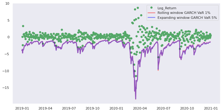
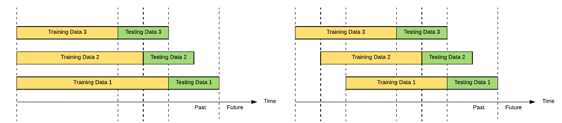
In the Fixed Rolling Window approach, new data are added while old ones are dropped from the sample

Expanding window

In the Expanding Window approach, new data are continuously added to the sample without dropped old data

Example of Evaluation
------------------------------------------------
Rolling Window Forcasting ARCH
Mean Absolute Error (MAE): 0.000113
Mean Absolute Percentage Error (MAPE): inf
Root Mean Square Error (RMSE): 0.000438
------------------------------------------------
Rolling Window Forcasting GARCH
Mean Absolute Error (MAE): 0.00014
Mean Absolute Percentage Error (MAPE): inf
Root Mean Square Error (RMSE): 0.0005
------------------------------------------------
Rolling Window Forcasting EGARCH
Mean Absolute Error (MAE): 0.000147
Mean Absolute Percentage Error (MAPE): inf
Root Mean Square Error (RMSE): 0.000518

Value at Risk (VaR) Forecasting and Backtesting

We can use the conditional variance given by the GARCH(1,1) model for the estimation of Value at Risk (VaR). For the underlined asset’s distribution properties we can use the specific distribution such as "normal", "t", "skewnormal", "skewt". For this method Value at Risk is expressed as: