Signal Separation

0.0.15 version

Version 0.0.15 enables the simplest generation and separation of analytical chemistry signals consisting of two Gaussian peaks 100 wide, 0.8 to 15 high, difference from 0 to 100. The signal length is 1000 points.

The algorithm is based on theoretical considerations about the signal function contained in the paper (see reference 1).

Features

• Genetic algorithm (see reference 2)
• Quick script for generating 1d-convolutional neural network architecture and training it (the possibility of setting the optimizer, seed, etc. in one line)
• Generation of a simple signal of two overlapping peaks with Gaussian distribution
• Modification of the cost function to compensate for the rarity of the data (see: reference 3)
• A script that estimates the positions and heights of peaks based on the generated signal (Uses CNN + SVR + Cost Modifications).

Installation

pip install signal_separation

import signal_separation as s

About ProjektInzynierski.ipynb and program.py

The ProjektInzynierski.ipynb file is an older, less polished, and safer version of the program. It can be run on the Google Colab platform. It uses the program.py file for its operation.

How to create signal

- a random variable with a normal distribution (mean: 0, std: 0.005)

- gaussian distribution density function (h - maximum value, t - horizontal coordinate of the maximum value, FWHM = 100)

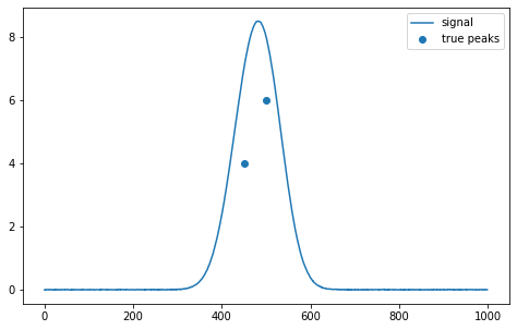
s.gensign(h1, h2, t1, t2) 

for example:

s.gensign(4, 6, 450, 500, return_y_values=False)

The resulting signal is the numpy.ndarray array and can be represented by the matplotlib library:

How to estimate signal parameters

In order to estimate, the signal must be provided (it can be simulated) as well as the trained network parameters and trained SVR.

model = s.create_network(s.only_after_act, 5)
svrh = s.download_svrh()
svrt = s.download_svrt()
s.download_weights(model)
estimation = s.predicting(model, svrh, svrt, signal)

Examples of estimated values (h1, h2, t_m1, t_m2):

>>> estimation
array([[  3.92313289,   6.10226897, 449.80370327, 500.51755778]])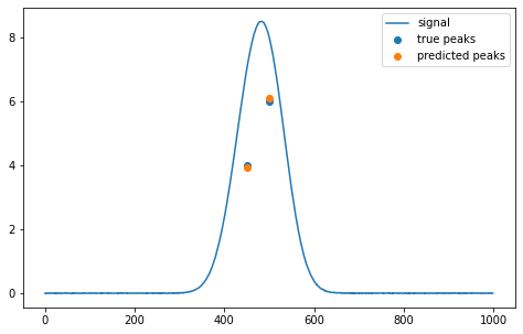

Other uses of the library

Training the neural network (with modification of the cost function)

import signal_separation as s
import numpy as np
import tensorflow as tf

Training and validation set

size = 50000
x_data = np.zeros([size,1000])
y_data = np.zeros([size,4])
for i in range(size):
  x_data[i,:], y_data[i,0], y_data[i,1], y_data[i,2], y_data[i,3] = s.gensign_random(0.8, 15, 400, 500, 10)
  
y_new = s.standardize(y_data, 400, 500, 400, 600, 0.8, 15)

x = x_data

size = y_new.shape[0]

y_new_test = y_new[:int(size*0.1),:]
x_t = x[:int(size*0.1),:]

y_new = y_new[int(size*0.1):,:]
x = x[int(size*0.1):,:]

Weight function

cost_height_prop = s.cost_function(s.ratio_of_uniforms, 0.8, 15, 1, s.height_ratio(s.destandardize_height(y_new[:,0], 0.8, 15),s.destandardize_height(y_new[:,1], 0.8, 15)), 0.00001)
cost_time2 = s.cost_function(s.sum_of_uniforms, 0.1, 0.9, 1, y_new[:,3], 0.00001)

Create an algorithm with input data: x_t, x; output data: y_new_test, y_new, and weight functions and train an algorithm with the hyperparameters (seed, network fork point, optimizer, base learning rate, position of the normalization batch layer).

train_network = s.train_network_maker(x_t, y_new_test, x, y_new, cost_height_prop, cost_time2)

model = train_network(2, 5, tf.keras.optimizers.Adam, 0.01, s.only_after_act)

You can estimate the model without using SVR if you enter None in the svrt and svrh values:

model = s.create_network(s.only_after_act, 5)
s.download_weights(model)
estimation = s.predicting(model, svrh=None, svrt=None, signal=signal)

>>> estimation
array([[  3.98014808,   5.80291796, 450.34817505, 501.23461914]])

Training the genetic algorithm

Definition of hyperparameters and population of the genetic algorithm

x = s.Population(5, 5)
x.define_feature(1, "random state", [1, 2, 3])
x.define_feature(2, "network fork point", [1,3,5,7])
x.define_feature(3, "optimizer", [tf.keras.optimizers.Adam,tf.keras.optimizers.SGD, tf.keras.optimizers.Adagrad])
x.define_feature(4, "base learning rate", [0.001, 0.01, 0.05, 0.1])
x.define_feature(5, "BatchNormalization", [s.no_batch, s.only_before_act, s.only_after_act, s.after_input, s.after_input_and_after_act, s.after_input_and_before_act])

Loading previously trained hyperparameters (optional)

x.load('Stored.csv', 'Current.csv')

Algorithm training

beg=0 #Change to 1 when you have already loaded the hyperparameter database and you do not want to reinitialize them
for itera in range(10):
  if beg==1:
    x.initialize()
    beg=0
  else:
    x.IndBeg()

  x.Check()
  for i in range(5):
    print(x.check_is_metric_wrote())
    if not x.check_is_metric_wrote(): #Checking whether there is already a counted metric in earlier individuals
      model = TrainNetwork(x.read(1), x.read(2), x.read(3), x.read(4), x.read(5))
      if not np.isnan(model.history['loss'][-1]):
        x.read_metric(-model.history['loss'][-1])
      else:
        x.read_metric(-100)
    x.nextind()

  x.store() #Saving in history
  print('Result:')
  print(x.initialized)
  x.sorting() #Sorting
  print('Sorted result:')
  print(x.initialized)
  x.selection() 
  print('Result after selection:')
  print(x.initialized)
  x.crossing()
  print('Result after crossing:')
  print(x.initialized)
  x.mutation(0.2) #Mutation with 20% mutation coefficient
  print('Result after mutation:')
  print(x.initialized)
  x.save()

CNN + SVR

By performing SVR on the feature vector, you can improve the neural network.

model = s.create_network(s.only_after_act, 5)
s.download_weights(model)

hvector = Model(inputs=model.input,
                                 outputs=model.layers[-5].output)
tvector = Model(inputs=model.input,
                                 outputs=model.layers[-4].output)

xt = tvector.predict(x)
xh = hvector.predict(x)

xt_t = tvector.predict(x_t)
xh_t = hvector.predict(x_t)

from sklearn.multioutput import MultiOutputRegressor
from sklearn.svm import SVR

svr = SVR(epsilon=0.001,  kernel='rbf', C=1, gamma=0.1)
svrh = MultiOutputRegressor(svr)
svrh.fit(xh, y_new[:, :2])
pred_train1 = svrh.predict(xh)
pred_test1 = svrh.predict(xh_t)

svrt = MultiOutputRegressor(svr)
svrt.fit(xt, y_new[:, 2:])
pred_train2 = svrt.predict(xt)
pred_test2 = svrt.predict(xt_t)

The resulting svrt and svrh can be used in the predicting function:

s.predicting(model, svrh, svrt, signal)

License

Free Software, made by Mieszko Pasierbek

References

[1] - J. Dubrovkin, „Mathematical methods for separation of overlapping asymmetrical peaks in spectroscopy and chromatography. Case study: one-dimensional signals”, International Journal of Emerging Technologies in Computational and Applied Sciences 11.1 (2015), 1–8.

[2] - T. Nagaoka, „Hyperparameter Optimization for Deep Learning-based Automatic Melanoma Diagnosis System”, Advanced Biomedical Engineering 9 (2020), 225

[3] - M. Steininger, K. Kobs, P. Davidson, A. Krause i A Hotho, „Density-based weighting for imbalanced regression”, Machine Learning 110 (2021), 2187–2211.