Business Analytics Study Guide

Niko Seino 2023-03-20

• Intro: What is Business Analytics?
• Descriptive Data Mining
  • Cluster Analysis
    • Measuring Similarity and Dissimilarity
    • Cluster Analysis Methods
• Predictive Data Mining
  • Linear Regression
    • Simple linear regression
    • Multiple Regression
  • Logistic Regression
    • Addressing Potential Issues
    • Performance Measures
• Time Series Analysis
  • Forecasting Methods
  • Assessing Forecast Accuracy

Intro: What is Business Analytics?

The scientific process of transforming data into insights for making better decisions. I.e., helping businesses improve processes, products, or services based on data.

Business decision-making process:

1. Identify the problem
2. Determine the criteria used to evaluate alternative solutions
3. Determine the set of alternative solutions
4. Evaluate the alternatives
5. Choose an alternative

Challenges to Decision Making:

1. Uncertainty
2. Overwhelming number of alternative solutions

BA Techniques:

1. Descriptive Analytics
   • Analyze past data to identify trends and patterns in that data
   • Examples: data queries, reports, data dashboards, data mining
2. Predictive Analytics
   • Use past data to predict the future or the impact of one variable on another
   • Examples: linear regression, time series analysis, simulation, data mining
3. Prescriptive Analytics
   • Suggest a course of action to take to solve a problem
   • Predictive analysis combined with a rule or set of rules (rule-based models)
   • Examples: optimization models, simulation optimization

Examples of analytics in different fields:

• Finance:
  • Create predictive models to forecast financial performance, asses risk of investment portfolios
  • Prescriptive models to construct optimal portfolios of investments, allocate assets, create optimal budgeting plans
• HR (People Analytics):
  • Assess factors that contribute to productivity, evaluate potential new hires
  • Forecast future employee turnover and retention
• Marketing:
  • Better understand consumer behavior through the use of scanner data, social media data
  • Determine more effective pricing strategies, improve forecasting of demand, increase customer satisfaction and loyalty
• Healthcare:
  • Improve facility scheduling, patient flow, purchasing, and inventory control
  • Prescriptive analytics for diagnosis and treatment
• Web Analytics:
  • Determine best ways to configure sites, position ads, and utilize social networks to promote products and services

Ethical Issues

• Analytics professionals have a responsibility to:
  • Protect data
  • Be transparent about how the data was collected and what it contains
  • Disclose methods used to analyze the data and any assumptions
  • Provide valid conclusions and understandable recommendations to their clients

Descriptive Data Mining

• Descriptive data-mining, AKA unsupervised learning:
  • no outcome variable to predict
  • goal is to use the variable values to identify relationships between observations
  • no definitive measure of accuracy–qualitative assessments assess and compare results

Cluster Analysis

• Goals is to break down a large group of observations into a smaller group with similar characteristics
  • observations within clusters are similar, and observations in different clusters are dissimilar
• Used in marketing to divide customers into homogeneous groups (e.g. demographics) in order to market more effectively to those groups (market segmentation)
• Can also be used to identify outliers

Measuring Similarity and Dissimilarity

For Numeric Variables:

• Euclidean Distance
  • Measure of dissimilarity
  • Straight line distance from point to point
  • Need to first standardize the units of each variable in order to compare them (i.e. find z-scores)
• Manhattan Distance
  • Measures distance as if traveling by city blocks
    • Sum of lengths of perpendicular line segments connecting observations u and v
  • Deals better with outliers and data with more dimensionality

Euclidean Distance Formula for observations u, v with q variables:

$$ d_uv = \sqrt{(u_1-v_1)^2+(u_2-v_2)^2+...(u_q-v_q)^2} $$

Manhattan Distance Formula:

$$ d_uv = |u_1-v_1|+|u_2-v_2|+...+|u_q-v_q| $$

For Categorical Variables:

Note: Categorical variables should be encoded as dummy variables, e.g. 0-1

• Matching Coefficient
  • Calculated by dividing the number of variables with matching values for observations u and v by the total number of variables
  • Might not always work with multiple variables, e.g. if two observations both have “0” value, it would be counted as a sign of similarity, even though the matching “0” values could mean different things
• Jaccard’s Coefficient
  • Emphasizes similar characteristics by only counting the 1’s, and not the 0’s.
  • Calculated by taking the number of variables with matching one values for u and v, divided by the total number of variables minus the number of matching zero values for u and v
  • Jaccard’s distance = 1-Jaccard’s Coefficient

Cluster Analysis Methods

• K-means Clustering
  • Used with numerical observations
  • Can deal with large datasets
  • Must first specify number of clusters needed, then assign observations to the nearest cluster
  • After all observations assigned to a cluster, the resulting cluster centroids are calculated
    • Centroid = the average observation of a cluster
  • Then, using updated cluster centroids, all observations are reassigned to cluster with closest centroid
  • This process repeats until there is no change in the clusters, or a specified max number of iterations is reached
  • At this point, can look at the groups and figure out the most interesting and relevant characteristics of each cluster
  • Determine strength of clusters by calculating ratio of between cluter centroid distance to the average within cluster distance
    • this ratio should be > 1 to indicate a useful cluster, because we want larger distance between clusters, and small distance within clusters
• Hierarchical Clustering
  • Unlike K-means, don’t need to know the number of clusters at the start
  • First, each observation is its own cluster, then iteratively clusters that are most similar are combined, decreasing the number of distinct clusters
  • Good for when you want to examine solutions with a wide range of clusters or observe how clusters are nested
  • Cons: sensitive to outliers, computationally expensive
  • Dissimilarity determined by calculating distance between observations in first cluster and observations in second cluster. This can be calculated using various methods:
    • Single Linkage
      • dissimilarity defined by distance between pairs of observations that are most similar
      • can result in long, elongated clusters
    • Complete Linkage
      • dissimilarity defined by distance between pairs of observations that are most different
      • creates cluster with mostly equal diameters, by can be distorted by outliers
    • Group Average Linkage
      • looks at average similarity among all possible pairs of observations between two clusters
      • produces clusters less dominated by dissimilarity between single pairs of observations
    • Ward’s Method
      • most commonly used method
      • only used with numerical variables
      • when merging two clusters, calculates the average observaion of all of the observations in two clusters, then calculates sum of squared distance from each observation in the new cluster to the centroid
      • results in a sequence of aggregated clusters that minimizes loss of information
  • Create a dendogram (tree diagram) to visually summarize output from hierarchical clustering
• Clustering mixed data (numerical and categorical)
  1. First apply hierarchical clustering to only the categorical variables and identify number of “first-step” clusters, then apply k-means clustering separately to the numerical variables using that number
  2. Numerically encode categorical variables (binary coding) and then standardize both categorical and numerical variable values

Predictive Data Mining

• Uses statistical models on current data to predict a future outcome
• In business, used to either estimate continuous outcomes, or classify categorical outcomes.
• Requires having a large data set with many variables

Linear Regression

Regression

• Models relationship between dependent variable (y) and 1 or more independent variables (x)
• Uses one variable to predict another
• Goal is to find the line of best fit that minimizes error between predicted values and observed values
  • To find line of best fit, calculate the sum of squared errors

$$SSE = \sum (y - \hat{y})^2$$

• Sum of Squared Errors: measures the difference between the model’s predictions and the actual values for y
  • Shows how well observations cluster around the regression line that predicts y
  • Best fitting line will have smallest possible SSE

Simple linear regression

$$ y = ß_0 + ß_1x + ε $$

ß0 = intercept ß1 = slope ε = error term (unexplained variability)

For an estimated regression equation, ε is dropped

• The slope indicates the average change in y with a one unit change in x.

• The intercept indicates the value expected for y when x is 0

• In R, use the lm() function to find slope coefficient and intercept. We can then use these values in our equation to make predictions

• Coefficient of Determination

  • In a simple linear regression: r^2
  • In a multiple regression: R^2
  • Calculated by taking the sum of squares due to regression and diving the total sum of squares (SSR/SST), or 1-sum of squared errors divided by total sum of squares (1-SSE/SST)
    • SST=How well observations cluster around the line that represents the mean of y
  • Always between 0 and 1: value closer to 1 indicates the model is better at predicting y values

Multiple Regression

$$ y = ß_0 + ß_1x_1 + ß_2x_2 + ... + ß_qx_q + ε $$

q = number of independent variables
ß0 = the mean of y when all of the x variables are 0, ß1 = the change in the mean value of y with a one unit increase in the ß1 variable, holding all other independent variables in the model constant

• Similar to simple linear regression, we want to find the model that results in the least errors
• Since the variables will have different units, use the lm() function to find slope coefficients, then standardize them by converting to z-scores
  • In R, can do this using lm.beta() from “lm.beta” package
  • Compare absolute value of the standardized coefficients to see which variable makes the strongest contribution to predicting y
• Note: Adding new variables to R^2 to a regression model will always increase R^2
  • To account for this, for multiple regressions we use an adjusted R^2 value

Possible issues with multiple regressions:

• Multicollinearity
  • when predictor variables are too correlated with each other to identify their specific contributions to predicting the outcome variable
  • slope coefficients for two highly correlated variables may change dramatically if they’re both included in the analysis; one variable may distort slope coefficient of the other
  • might change p-value, or statistical significance of correlated slope coefficients
  • best way to assess multicollinearity: variance inflation factor (VIF)
    • measures how much standard errors of regression coefficients increase when multicollinearity exists
    • we want VIF of a variable to be as close to 1 as possible (1=no correlation between that predictor and the other predictor variables)
    • VIF of 4 needs further consideration; VIF of 10 suggests serious multicollinearity
    • In R, can calculate VIF using VIF() function from “car” package
    • Can also use cor() function to create a correlation matrix and view correlations between pairs of variables. Correlation > .7 indicates possible multicollinearity and should consider removing one of the variables from regression analysis.
• Overfitting
  • Fitting the model too closely to the sample data, resulting in a model that does not accurately reflect the population
  • Can indicate too many predictor variables in our model
    • To prevent this, use random sampling to build a training set and test the model with a validation set
    • Typically use 70% of the data for training, 30% for validation
    • In R, can use the ols_step_all_possible() function from the “olsrr” package on our regression model with all predictor variables from our training set. This will show the R^2 values for all combinations of the variables, so we can see which combination has the hightest R^2. It will also show AIC values, which is a good measure of model fit.
      • The predictors with the lowest AIC value will be the best ones to use in our regression
    • After determining best predictor variables to use, run another multiple regression using those variables and our validation data frame
    • Finally, we can use the coefficients from this regression analysis to construct a regression equation that can be used to make predictions

Logistic Regression

• Used if the outcome we are predicting is categorical, not continuous
• Predicting probability, or likelihood of the outcome
  • Examples: Predict whether an applicant will or will not default on a loan
  • Predict whether new employees will accept job offers based on salary and benefits
  • Predict whether or not a customer will make a claim based on certain characteristics
• Instead of predicting a y value, predicting the log odds
• In a logistic regression summary, the coefficient tells us the average change in the log odds of the outcome, given a 1-unit change in the predictor variable

Given probability (p), odds = p/1-p; so the logistic regression equation is:

$$ ln(\hat{p}/1-\hat{p}) = ß_0 + ß_1x_1 + ß_2x_2 + ... + ß_qx_q $$

Addressing Potential Issues

Data Partitioning

• Once a data sample has been prepared for analysis, it should be partitioned into 2 or 3 sets to appropriately evaluate the performance of data mining models (Static Holdout Method)
  1. Training set - used to build the model (see which variables best predict outcome)
  2. Validation set - try a few of the best models
  3. Testing Set - run the best model

Class Imbalance

• With a binary outcome variable, the outcomes fall into either a majority class or minority class. Class imbalance occurs when there were many more observations falling into one class than another. Ways to address this:
  1. Undersampling - randomly sample fewer observations from majority class, and use all observations from minority class
     • con: may not capture important information from majority class
  2. Oversampling - use all or most observations from majority class, and random sample of minority class with replacement (i.e. making copies of the minority class observations)
     • con: may create a data set that doesn’t accurately reflect the original
  3. Random Oversampling Examples (ROSE) - uses bootstrapping to create a synthetic training set with a balanced number of observations in each class

Performance Measures

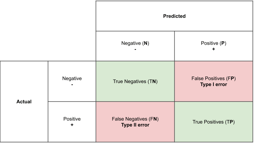
• Set a probability cuttoff (usually .5) that will determine into which category an observation will fall
• Classification error is commonly displayed in a confusion matrix, which tells how many outcomes the model got right and wrong
  • Overall error rate = # of incorrectly predicted outcomes / total # of outcomes x 100
  • Accuracy = 1-overall error rate
  • Rate of correctly predicting a positive = sensitivity
  • Rate of correctly predicting a negative = specificity

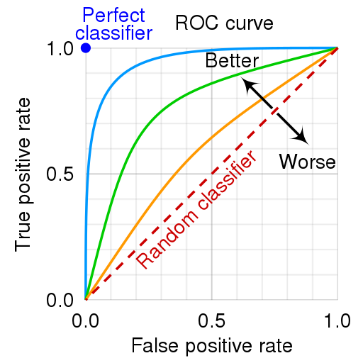
• Receiver Operating Characteristic (ROC) Curve: graphical approach to showing trade offs of model’s ability to correctly predict positives to negatives
  • Has error rate of predicting a negative on the x-axis, and true positive (sensitivity) rate on the y-axis
  • Evaluate the area under the ROC curve (AUC)
    • Larger AUC = better classifier; means we would not see the classifications in our model by random chance

Logistic Regression Summary:

1. Create your test, training, and validation data sets
2. Test for imbalance by creating undersample, oversample, and ROSE sets
3. Perform logistic regressions on each set
4. Generate confusion matrices for each regression
5. Obtain probabilities for each observation in the validation set
6. Attach these probabilities to the validation dataframe
7. Obtain predicted class for each observation and attach to the validation dataframe
8. Apply the best model to the test set

Time Series Analysis

Forecasting

• Predicting the future state of some key variable in order to predict future values of quantitative data
• Used to project future sales, revenue, employment, seasonal buying trends, best times to run promotions, etc.
• Example business questions related to forecasting:
  • What will the demand for a business product be next year?
  • How will revenue be affected by different seasons?
• Can be done when there is past data available, the information can be quantified, and it is reasonable to assume that past patterns will continue into the future.
  • Time Series : A sequence of observations on a variable that occur at equally spaced time intervals
    • Objective is to uncover a pattern in the time series and extrapolate the pattern to forecast the future
    • First step is to construct a time series plot to graph the relationship between time (x-axis) and the time series variable (y-axis). The type of pattern plotted will dictate which forecasting method to use.

Time Series Patterns

• Horizontal:
  • Data fluctuate randomly around a constant mean over time
  • Variability is also constant over time
• Trend Pattern:
  • Data shows gradual shifts to relatively higher or lower values over a period of time
  • Usually the result of long-term factors e.g. population growth, shifting demographics, improving technology, changes in customer preferences
• Seasonal Pattern:
  • Data shows recurring patterns over successive periods of time
  • e.g. each year, a bathing suit retailer expects sales to dip in fall and winter months, and peak in spring and summer months
• Trend and Seasonal:
  • A time series that has both trend and seasonal patterns
  • e.g. a smartphone’s companies sales show an overall increasing trend, but also show sales are lowest in second quarter of each year, and highest in fourth quarter.
• Cyclical:
  • Time series plot shows alternating sequence of points below and above the trendline that lasts for more than one year
  • Often occurs due to multiyear business cycles
  • e.g. periods of moderate inflation followed by rapid inflation
  • Can be extremely difficult to forecast

Forecasting Methods

For time series data with horizontal patterns:

1. Naive forecasting

• Simply uses the previous time interval’s value as the forecast for the next time interval; e.g. if forecasting weekly sales, the sales value from week 1 is used as the forecast for week 2.

2. Moving Averages

• Uses the average of the most recent data values in the time series as the forecast for the next period.
• When a new observation becomes available, it replaces the oldest observation and a new average is computed; therefore, the average moves with each new period.

3. Exponential Smoothing

• Uses a weighted average of past time series values as a forecast
• Weight is denoted by a smoothing constant, α
  • A large α will give more weight to most recent observations (less smoothing), while a small α will give more attention to past observations (more smoothing)
• Exponential Smoothing Formula:

$$\hat{y}_{t+1} = αy_t + (1-α)\hat{y}_t$$

• The forecast for period t + 1 is equal to the weighted average of the actual value in period t plus the forecast for period t

For Time Series Data with trend, seasonal pattern, or both:

1. Linear Trend Projection:

• Uses linear regression analysis to find the best-fitting line to fit the data. Equation is similar to any other linear regression:

$$ \hat{y}_t = ß_0 + ß_1t $$

y = the forecast of sales in period t t = time period bo = y-intercept b1 = the slope

• Compute the estimated slope and intercept using Excel or R, then use those values to predict observations.

• When the data has seasonality without trend, add dummy variables to the model to code the seasons (e.g. Q1, Q2, Q3, Q4 for quarterly trend).

  • One of the variables (e.g. Q1) will be used as a reference to which all other dummy variables (Q2, Q3, Q4) will be compared.
  • The regression equation becomes:

$$ \hat{y}_t = ß_0 + ß_1{Qtr1}_t + b_2{Qtr2}_t + b_3{Qtr3}_t $$

• When the data has seasonality with trend, combine the previous two approaches, which results in the following equation:

$$ \hat{y}_t = ß_0 + ß_1{Qtr1}_t + b_2{Qtr2}_t + b_3{Qtr3}t + b{4t}$$

Assessing Forecast Accuracy

Forecast Error: the difference between the actual and the forecasted values for period t

$$ e_t = y_t - \hat{y}_t $$

• A positive error means the forecast method underestimated the actual value, negative means it overestimated

Mean Absolute Error (MAE): The average of the absolute values of the forecast errors.

• We take the absolute value so the positive and negative errors don’t offset each other.

$$ MAE = \sum{|e_t|}/n-k $$

Mean Squared Error (MSE): Similar to MAE, but instead of taking the absolute values, we square the errors

$$ MSE = \sum{e_t}^2/n-k $$

• We may also use Root Mean Squared Error (RMSE), which is the square root of the MSE.

Mean Absolute Percentage Error (MAPE): Calculates forecast error as a percentage of the actual sales value, which allows us to compare across different time units, or across different types of products.

$$ MAPE = \sum{|(e_t/y_t)100|}/n-k $$

• We can use these accuracy measures to compare different forecasting methods and choose the one with the lowest error values.