【Hackathon 5th No.57】Neural networks for topology optimization

docs/zh/examples/topopt.md

@@ -0,0 +1,318 @@
+# TopOpt
+
+<a href="https://aistudio.baidu.com/projectdetail/6956236" class="md-button md-button--primary" style>AI Studio快速体验</a>
+
+=== "模型训练命令"
+
+    ``` sh
+    python topopt.py
+    ```
+
+=== "模型评估命令"
+
+    ``` sh
+    python topopt.py 'mode=eval' 'EVAL.pretrained_model_path_dict={"Uniform": "path1",  "Poisson5": "path2",  "Poisson10": "path3",  "Poisson30": "path4"}'
+    ```
+
+## 1. 背景简介
+
+拓扑优化 (Topolgy Optimization) 是一种数学方法，针对给定的一组负载、边界条件和约束，在给定的设计区域内，以最大化系统性能为目标优化材料的分布。这个问题很有挑战性因为它要求解决方案是二元的，即应该说明设计区域的每个部分是否存在材料或不存在。这种优化的一个常见例子是在给定总重量和边界条件下最小化物体的弹性应变能。随着20世纪汽车和航空航天工业的发展，拓扑优化已经将应用扩展到很多其他学科：如流体、声学、电磁学、光学及其组合。SIMP (Simplied Isotropic Material with Penalization) 是目前广泛传播的一种简单而高效的拓扑优化求解方法。它通过对材料密度的中间值进行惩罚，提高了二元解的收敛性。
+
+
+## 2. 问题定义
+
+拓扑优化问题：
+
+$$
+\begin{aligned}
+& \underset{\mathbf{x}}{\text{min}} \quad && c(\mathbf{u}(\mathbf{x}), \mathbf{x}) = \sum_{j=1}^{N} E_{j}(x_{j})\mathbf{u}_{j}^{\intercal}\mathbf{k}_{0}\mathbf{u}_{j} \\
+& \text{s.t.} \quad && V(\mathbf{x})/V_{0} = f_{0} \\
+& \quad && \mathbf{K}\mathbf{U} = \mathbf{F} \\
+& \quad && x_{j} \in \{0, 1\}, \quad j = 1,...,N
+\end{aligned}
+$$
+
+其中：$x_{j}$ 是材料分布 (material distribution)；$c$ 指可塑性 (compliance)；$\mathbf{u}_{j}$ 是 element displacement vector；$\mathbf{k}_{0}$ 是 element stiffness matrix for an element with unit Youngs modulu；$\mathbf{U}$, $\mathbf{F}$ 是 global displacement and force vectors；$\mathbf{K}$ 是 global stiffness matrix；$V(\mathbf{x})$, $V_{0}$ 是材料体积和设计区域的体积；$f_{0}$ 是预先指定的体积比。
+
+## 3. 问题求解
+
+实际求解上述问题时为做简化，会把最后一个约束条件换成连续的形式：$x_{j} \in [0, 1], \quad j = 1,...,N$。 常见的优化算法是 SIMP 算法，它是一种基于梯度的迭代法，并对非二元解做惩罚：$E_{j}(x_{j}) = E_{\text{min}} + x_{j}^{p}(E_{0} - E_{\text{min}})$，这里我们不对 SIMP 算法做过多展开。由于利用 SIMP 方法, 求解器只需要进行初始的 $N_{0}$ 次迭代就可以得到与结果的最终结果非常相近的基本视图，本案例希望通过将 SIMP 的第 $N_{0}$ 次初始迭代结果与其对应的梯度信息作为 Unet 的输入，预测 SIMP 的100次迭代步骤后给出的优化解。
+
+### 3.1 数据集准备
+
+数据集为整理过的合成数据：[下载地址](https://aistudio.baidu.com/datasetdetail/245115/0)  
+整理后的格式为 `"iters": shape = (10000, 100, 40, 40)`，`"target": shape = (10000, 1, 40, 40)`
+
+- 10000 - 随机生成问题的个数
+
+- 100 - SIMP 迭代次数
+
+- 40 - 图像高度
+
+- 40 - 图像宽度
+
+
+数据集地址请存储于 `./datasets/top_dataset.h5`  
+
+生成训练集：原始代码利用所有的10000问题生成训练数据。
+
+``` py linenums="68"
+--8<--
+examples/topopt/functions.py:68:101
+--8<--
+```
+
+``` py linenums="39"
+--8<--
+examples/topopt/topopt.py:39:48
+--8<--
+```
+
+### 3.2 模型构建
+
+经过 SIMP 的 $N_{0}$ 次初始迭代步骤得到的图像 $I$ 可以看作是模糊了的最终结构。由于最终的优化解给出的图像 $I^*$ 并不包含中间过程的信息，因此 $I^*$ 可以被解释为图像 $I$ 的掩码。于是 $I \rightarrow I^*$ 这一优化过程可以看作是二分类的图像分割或者前景-背景分割过程，因此构建 Unet 模型进行预测，具体网络结构如图所示：
+![Unet](https://ai-studio-static-online.cdn.bcebos.com/7a0e54df9c9d48e5841423546e851f620e73ea917f9e4258aefc47c498bba85e)
+
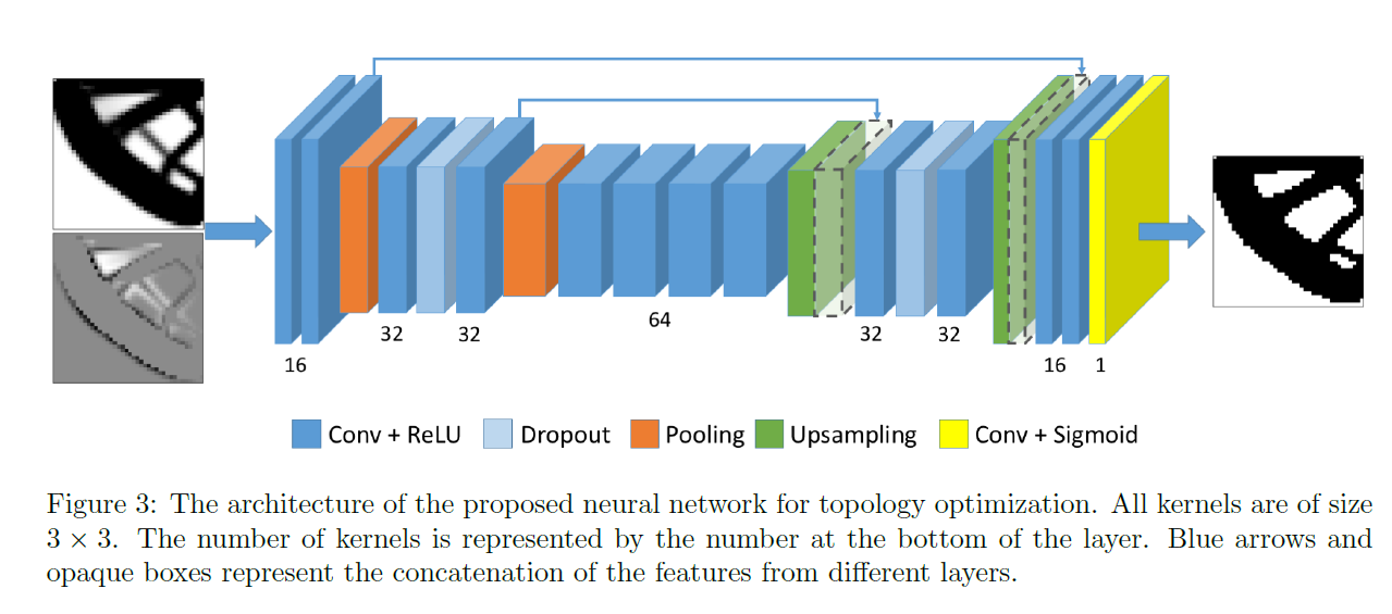+``` py linenums="89"
+--8<--
+examples/topopt/topopt.py:89:92
+--8<--
+```
+这里 `assert` 的原因是论文中已给出模型的参数量为 192113, 此处做以验证。
+
+详细的模型代码在 `examples/topopt/TopOptModel.py` 中。
+
+
+### 3.3 参数设定
+
+根据论文以及原始代码给出以下训练参数：
+
+``` yaml linenums="49"
+--8<--
+examples/topopt/conf/topopt.yaml:49:58
+--8<--
+```
+
+``` py linenums="35"
+--8<--
+examples/topopt/topopt.py:35:38
+--8<--
+```
+
+
+### 3.4 transform构建
+
+根据论文以及原始代码给出以下自定义 transform 代码，包括随机水平或垂直翻转和随机90度旋转，对 input 和 label 同时 transform：
+
+``` py linenums="102"
+--8<--
+examples/topopt/functions.py:102:133
+--8<--
+```
+
+
+### 3.5 约束构建
+
+在本案例中，我们采用监督学习方式进行训练，所以使用监督约束 `SupervisedConstraint`，代码如下：
+
+``` py linenums="49"
+--8<--
+examples/topopt/topopt.py:49:75
+--8<--
+```
+
+`SupervisedConstraint` 的第一个参数是监督约束的读取配置，配置中 `"dataset"` 字段表示使用的训练数据集信息，其各个字段分别表示：
+
+1. `name`： 数据集类型，此处 `"NamedArrayDataset"` 表示分 batch 顺序读取的 `np.ndarray` 类型的数据集；
+2. `input`： 输入变量字典：`{"input_name": input_dataset}`；
+3. `label`： 标签变量字典：`{"label_name": label_dataset}`；
+4. `transforms`： 数据集预处理配，其中 `"FunctionalTransform"` 为用户自定义的预处理方式。
+
+读取配置中 `"batch_size"` 字段表示训练时指定的批大小，`"sampler"` 字段表示 dataloader 的相关采样配置。
+
+第二个参数是损失函数，这里使用[自定义损失](#381)，通过 `cfg.vol_coeff` 确定损失公式中 $\beta$ 对应的值。
+
+第三个参数是约束条件的名字，方便后续对其索引。此次命名为 `"sup_constraint"`。
+
+在约束构建完毕之后，以我们刚才的命名为关键字，封装到一个字典中，方便后续访问。
+
+
+### 3.6 采样器构建
+
+原始数据有100个通道对应的是 SIMP 算法 100 次的迭代结果，本案例模型目标是用 SIMP 中间某一步的迭代结果直接预测 SIMP 最后一步的迭代结果，而论文原始代码中的模型输入是原始数据对通道进行采样后的数据，为应用 PaddleScience API，本案例将采样步骤放入模型的 forward 方法中，所以需要传入不同的采样器。
+
+``` py linenums="23"
+--8<--
+examples/topopt/functions.py:23:67
+--8<--
+```
+
+``` py linenums="79"
+--8<--
+examples/topopt/topopt.py:79:81
+--8<--
+```
+
+### 3.7 优化器构建
+
+训练过程会调用优化器来更新模型参数，此处选择 `Adam` 优化器。
+
+``` py linenums="93"
+--8<--
+examples/topopt/topopt.py:93:97
+--8<--
+```
+
+### 3.8 loss和metric构建
+
+#### 3.8.1 loss构建
+损失函数为 confidence loss + beta * volume fraction constraints:
+
+$$
+\mathcal{L} = \mathcal{L}_{\text{conf}}(X_{\text{true}}, X_{\text{pred}}) + \beta * \mathcal{L}_{\text{vol}}(X_{\text{true}}, X_{\text{pred}})
+$$  
+
+confidence loss 是 binary cross-entropy:  
+
+$$
+\mathcal{L}_{\text{conf}}(X_{\text{true}}, X_{\text{pred}}) = -\frac{1}{NM}\sum_{i=1}^{N}\sum_{j=1}^{M}\left[X_{\text{true}}^{ij}\log(X_{\text{pred}}^{ij}) +  (1 - X_{\text{true}}^{ij})\log(1 - X_{\text{pred}}^{ij})\right]
+$$  
+
+volume fraction constraints:  
+
+$$
+\mathcal{L}_{\text{vol}}(X_{\text{true}}, X_{\text{pred}}) = (\bar{X}_{\text{pred}} - \bar{X}_{\text{true}})^2
+$$  
+
+loss 构建代码如下：
+
+``` py linenums="259"
+--8<--
+examples/topopt/topopt.py:259:274
+--8<--
+```
+
+#### 3.8.2 metric构建
+本案例原始代码选择 Binary Accuracy 和 IoU 进行评估:  
+
+$$
+\text{Bin. Acc.} = \frac{w_{00}+w_{11}}{n_{0}+n_{1}}
+$$
+
+$$
+\text{IoU} = \frac{1}{2}\left[\frac{w_{00}}{n_{0}+w_{10}} + \frac{w_{11}}{n_{1}+w_{01}}\right]
+$$
+
+其中 $n_{0} = w_{00} + w_{01}$ ， $n_{1} = w_{10} + w_{11}$ ，$w_{tp}$ 表示实际是 $t$ 类且被预测为 $p$ 类的像素点的数量
+metric 构建代码如下：
+
+``` py linenums="275"
+--8<--
+examples/topopt/topopt.py:275:317
+--8<--
+```
+
+
+### 3.9 模型训练
+
+本案例根据采样器的不同选择共有四组子案例，案例参数如下：
+
+``` yaml linenums="29"
+--8<--
+examples/topopt/conf/topopt.yaml:29:31
+--8<--
+```
+
+训练代码如下：
+
+``` py linenums="76"
+--8<--
+examples/topopt/topopt.py:76:113
+--8<--
+```
+
+
+### 3.10 评估模型
+
+对四个训练好的模型，分别使用不同的通道采样器 (原始数据的第二维对应表示的是 SIMP 算法的 100 步输出结果，统一取原始数据第二维的第 5，10，15，20，...，80 通道以及对应的梯度信息作为新的输入构建评估数据集) 进行评估，每次评估时只取 `cfg.EVAL.num_val_step` 个 bacth 的数据，计算它们的平均 Binary Accuracy 和 IoU 指标；同时评估结果需要与输入数据本身的阈值判定结果 (0.5作为阈值) 作比较。具体代码请参考[完整代码](#4)
+
+
+#### 3.10.1 评估器构建
+为应用 PaddleScience API，此处在每一次评估时构建一个评估器 SupervisedValidator 进行评估：
+
+``` py linenums="214"
+--8<--
+examples/topopt/topopt.py:214:241
+--8<--
+```
+
+评估器配置与 [约束构建](#35) 的设置类似，读取配置中 `"num_workers"：0` 表示单线程读取；评价指标 `"metric"` 为自定义评估指标，包含 Binary Accuracy 和 IoU。
+
+
+### 3.11 评估结果可视化
+
+使用 `ppsci.utils.misc.plot_curve()` 方法直接绘制 Binary Accuracy 和 IoU 的结果：
+
+``` py linenums="185"
+--8<--
+examples/topopt/topopt.py:185:195
+--8<--
+```
+
+
+## 4. 完整代码
+
+``` py linenums="1" title="topopt.py"
+--8<--
+examples/topopt/topopt.py
+--8<--
+```
+
+``` py linenums="1" title="functions.py"
+--8<--
+examples/topopt/functions.py
+--8<--
+```
+
+``` py linenums="1" title="TopOptModel.py"
+--8<--
+examples/topopt/TopOptModel.py
+--8<--
+```
+
+
+## 5. 结果展示
+
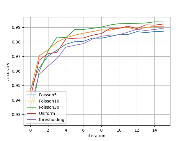
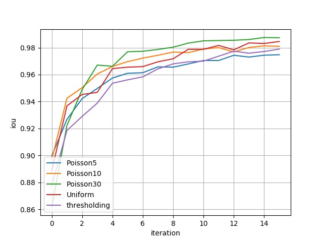
+下图展示了4个模型分别在16组不同的评估数据集上的表现，包括 Binary Accuracy 以及 IoU 这两种指标。其中横坐标代表不同的评估数据集，例如：横坐标 $i$ 表示由原始数据第二维的第 $5\cdot(i+1)$ 个通道及其对应梯度信息构建的评估数据集；纵坐标为评估指标。`thresholding` 对应的指标可以理解为 benchmark。
+
+<figure markdown>
+  ![bin_acc](https://ai-studio-static-online.cdn.bcebos.com/859ca7c5d6bb4d60b4e1a329b369c3f2bb942ba281664d1a9156397a34a9191b){ loading=lazy }
+  <figcaption>Binary Accuracy结果</figcaption>
+</figure>
+
+<figure markdown>
+  ![iou](https://ai-studio-static-online.cdn.bcebos.com/807ea645100447818d0bafc39e9d489eef26b7a0195d4bd59da4e68445d304cb){ loading=lazy }
+  <figcaption>IoU结果</figcaption>
+</figure>
+
+结果与[原始代码结果](https://github.com/ISosnovik/nn4topopt/blob/master/results.ipynb)基本一致
+
+此外将这些计算的指标与论文中展示的对应指标 (`table 1` 与 `table2` 中的) 对比，指标相对误差均小于 10%，以下表格是所有的指标计算结果：
+
+| bin_acc | eval_dataset_ch_5 | eval_dataset_ch_10 | eval_dataset_ch_15 | eval_dataset_ch_20 | eval_dataset_ch_25 | eval_dataset_ch_30 | eval_dataset_ch_35 | eval_dataset_ch_40 | eval_dataset_ch_45 | eval_dataset_ch_50 | eval_dataset_ch_55 | eval_dataset_ch_60 | eval_dataset_ch_65 | eval_dataset_ch_70 | eval_dataset_ch_75 | eval_dataset_ch_80 |
+| :---: | :---: | :---: | :---: | :---: | :---: | :---: | :---: | :---: | :---: | :---: | :---: | :---: | :---: | :---: | :---: | :---: |
+| Poisson5 | 0.9471 | 0.9619 | 0.9702 | 0.9742 | 0.9782 | 0.9801 | 0.9803 | 0.9825 | 0.9824 | 0.9837 | 0.9850 | 0.9850 | 0.9870 | 0.9863 | 0.9870 | 0.9872 |
+| Poisson10 | 0.9457 | 0.9703 | 0.9745 | 0.9798 | 0.9827 | 0.9845 | 0.9859 | 0.9870 | 0.9882 | 0.9880 | 0.9893 | 0.9899 | 0.9882 | 0.9899 | 0.9905 | 0.9904 |
+| Poisson30 | 0.9257 | 0.9595 | 0.9737 | 0.9832 | 0.9828 | 0.9883 | 0.9885 | 0.9892 | 0.9901 | 0.9916 | 0.9924 | 0.9925 | 0.9926 | 0.9929 | 0.9937 | 0.9936 |
+| Uniform | 0.9410 | 0.9673 | 0.9718 | 0.9727 | 0.9818 | 0.9824 | 0.9826 | 0.9845 | 0.9856 | 0.9892 | 0.9892 | 0.9907 | 0.9890 | 0.9916 | 0.9914 | 0.9922 |
+
+| iou | eval_dataset_ch_5 | eval_dataset_ch_10 | eval_dataset_ch_15 | eval_dataset_ch_20 | eval_dataset_ch_25 | eval_dataset_ch_30 | eval_dataset_ch_35 | eval_dataset_ch_40 | eval_dataset_ch_45 | eval_dataset_ch_50 | eval_dataset_ch_55 | eval_dataset_ch_60 | eval_dataset_ch_65 | eval_dataset_ch_70 | eval_dataset_ch_75 | eval_dataset_ch_80 |
+| :---: | :---: | :---: | :---: | :---: | :---: | :---: | :---: | :---: | :---: | :---: | :---: | :---: | :---: | :---: | :---: | :---: |
+| Poisson5 | 0.8995 | 0.9267 | 0.9421 | 0.9497 | 0.9574 | 0.9610 | 0.9614 | 0.9657 | 0.9655 | 0.9679 | 0.9704 | 0.9704 | 0.9743 | 0.9730 | 0.9744 | 0.9747 |
+| Poisson10 | 0.8969 | 0.9424 | 0.9502 | 0.9604 | 0.9660 | 0.9696 | 0.9722 | 0.9743 | 0.9767 | 0.9762 | 0.9789 | 0.9800 | 0.9768 | 0.9801 | 0.9813 | 0.9810 |
+| Poisson30 | 0.8617 | 0.9221 | 0.9488 | 0.9670 | 0.9662 | 0.9769 | 0.9773 | 0.9786 | 0.9803 | 0.9833 | 0.9850 | 0.9853 | 0.9855 | 0.9860 | 0.9875 | 0.9873 |
+| Uniform | 0.8887 | 0.9367 | 0.9452 | 0.9468 | 0.9644 | 0.9655 | 0.9659 | 0.9695 | 0.9717 | 0.9787 | 0.9787 | 0.9816 | 0.9784 | 0.9835 | 0.9831 | 0.9845 |
+
+## 参考文献
+* [Sosnovik I, & Oseledets I. Neural networks for topology optimization](https://arxiv.org/pdf/1709.09578)
+* [原始代码](https://github.com/ISosnovik/nn4topopt/blob/master/)