Additional information
Mantis uses several default data sources, to stop using these data sources add NA to the default path you'd like to stop using, for example: nog_ref_folder=NA
The default reference data sources are:
- Pfam
- KOfam
- eggNOG
- NCBI's protein family models (NPFM)
- Transporter classification database (TCDB)
It also uses a list of essential genes to identify HMM profile matches that correspond to previously identified essential genes.
To identify the taxonomic lineage it uses NCBI's taxonmic lineage found here.
A general reference is created for the eggNOG and NPFM compendiums, this general reference contains all the non-redundant information from the top level NCBI taxons: 2157 (Archaea), 2 (Bacteria), 2759 (Eukaryota), 10239 (Viruses), 28384 (Others), and 12908 (Unclassified).
Respective citations can be found in References and Acknowledgements
NPFM and eggNOG can use taxonomic lineage for taxa-specific functional annotation. Both rely on NCBI IDs, and so taxonomic lineage can determined in several manners:
- If a NCBI ID is provided, taxonomic lineage is calculated directly
- If a NCBI taxon name is provided, Mantis will query NCBI and retrieve the corresponding NCBI, and then calculate the respective taxonomic lineage
- If a GTDB taxon name or lineage is provided, Mantis first maps the GTDB information to NCBI. Since multiple NCBI may map to GTDB, we determine the lowest common ancestor (LCA) for all the mapped NCBI IDs. The final taxonomic lineage will correspond to the lineage of the LCA
We have found that setting the e-value to 1e-3 produces the best results with HMMER. While this values gives a bigger list of hits, the most significant hits are still selected. When using the Diamond homology search, the e-value threshold is set to dynamic by default as it was found to be optimal. The'dynamic' threshold changes according to the query sequence length, such that the e-value threshold correspond to 1e-sequence length/10
This can however be set to another value by adding -et evalue.
In HMMER and Diamond, the resulting e-value is scaled to sample size. For HMMER, hmmsearch is used; hmmsearch is automatically scaled to e-value (if doing homology search for a chunk, the e-value is divided by the chunk size and then multiplied by the original sample size). For Diamond, the e-value is first scaled by using Diamond's blastp with --dbsize 1 and then multiplying it by the number of residues in the original sample.
Possible combinations of hits are generated using the depth-first search (DFS) algorithm.
Combination of hits are chosen according to 3 different metrics, according to what defines a "good combination":
- High coverage;
- Low e-value;
- Low number of hits per combinations - many small sized hits are less significant than a few large sized hits;
This is defined by the following equation:
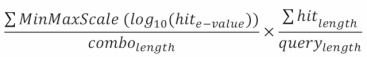
The left fraction's numerator depicts scaled e-value, the denominator the number of hits.
The right fraction depicts the coverage (percentage of the query sequence covered by our combination) of the combination of hits.
This score ranges from 0 to 1, 1 being the highest.
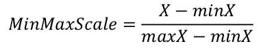
The e-values within our threshold are extremely low, making comparisons between the raw e-values meaningless. By using the log10 we reduce the range of this distribution, allowing comparison. This also avoids the precision loss that is inherent to the arithmetic capacities of all computer systems.
Other scaling equations could be applied, but the MinMaxScale transforms our e-values into proportions, which fits well the combination hit score calculation equation used.
The total amount of possible combinations (discarding the empty combination) is 2N-1 where N is the amount of hits our query has. Calculating and evaluating all possible combinations is not computationally feasible:
- 10 hits: 210 - 1 = 1023
- 15 hits: 215 - 1 = 32767
- 30 hits: 230 - 1 = 1073741823
When dealing with queries with a large number of hits, testing (and even generating) all combinations is not feasible. The adapted algorithm is as follows:
- Create an initial list of possible combinations - where the combination root is a query hit
- For each possible combination test possible hits that can be added
- Can combination be expanded? Go to 2; otherwise go to 4
- Return possible combinations
However, there are cases when this improved algorithm may not be feasible either (even with Cython):
- Long query sequence
- Low hit coverage
- High number of hits
If the previous algorithm doesn't finish within 1 minute, another algorithm (heuristic) comes into play:
- Select lowest e-value hit and add it to the combination.
- Does hit overlap with our combination? If not, add it to combination
- Are there any hits left? If yes go to 1.
To see how this works, check MANTIS_Processor.py.
The user is free to select from the 3 different hit processing algorithms dfs,heuristic, and bpo. The first two were previously introduced, the bpo algorithm only selects the most significant hit (potentially ignoring multiple domains).
The dfs provides the best results, however the heuristic is close behind, therefore for shorter runtimes we advise running the latter.
As previously explained, Mantis can get non-overlapping hits from the same reference. However, since Mantis uses a lot of different references, there might not be a consensus between them.
That is why it is crucial to find a way to find some sort of consensus between the different references.
The initial step is consists in pooling all sequence hits together, and finding the best combination. The best combination uses the same equation from Intra-reference hit processing. However, 3 additional variables are added, Hit consistency, reference weight, and Metadata quality.
Hit consistency corresponds to the amount of hits (among all hits) that have metadata consistent with the hits in the current combination of hits. reference weight refers to the average weight of all references in the current combination of hits (the weight can be customized by the user). Metadata quality corresponds to the average metadata quality of all the hits in the combination (0.25 for hits without any metadata, 0.5 for hits with only a free-text functional description in their metadata, 0.75 for hits with IDs in their metadata, 1 for hits that contain IDs and free-text functional descriptions in their metadata).
Metadata consistency is found in two manners:
- Consensus between identifiers
- Consensus between free-text description
The first is done through a pairwise comparison of the IDs within hits metadata. If the hits share IDs (e.g. hit 1 contains ID1, hit 2 contains ID1 and ID2), then they are considered to be describing the same function, and will thus be merged during the consensus generation. Since some reference sources use an hierarchical approach to IDs, we set a limit of up to 10 IDs of the same type (e.g. gene ontology ID). As an example, if we were to compare two annotations (from different references), one having 8 gene ontology IDs, the other 3, and each having 1 Pfam ID; during this step the gene ontology IDs would not be used for the consistency check between the references since the one of the annotations may contain unspecific IDs (e.g. gene ontology ID 0003674 - "molecular function"), instead only the Pfam ID would be compared. This avoids merging annotations with non-specific identifiers. If no consistency of IDs is found then the free-text functional description are compared with UniFunc. This tool outputs a similarity score, pairs of hits with a score above 0.9 are considered to be describing the same function.
After selecting the best combination of hits, each hit in the combination is expanded by merging it with other hits with consistent metatata.
Important Hit consistency is restricted to hits that have at least 70% residues overlap (can be customized)
To see how this works, check MANTIS_Consensus.py.
Mantis was built to be highly efficient and scalable, while at the same time not relying on heuristic techniques. There are several factors that can cause execution bottlenecks, some of which can be circumvented.
What are the efficiency bottlenecks?
- Workflow design – the workflow used is the main contributor to poor performance, an iterative approach is simple to implement but substantially inferior to a parallelized implementation.
- Number of cores - the number of cores influences speed performance the most, speed scales linearly with the number of cores, this depends on the hardware available;
- Number of processes - one would expect the ideal number of processes to be the same as the number of cores. Up to a certain point increasing the number of processes leads to speed gains, after around 2-3 times the number of cores there’s no more speed gain, increasing past this point can actually lead to severe efficiency decreases due to the overhead generated.
- Sample size – a larger search space (more query sequences to compare against reference profiles) translates into a higher runtime. An iterative execution can’t possibly handle metagenomic samples in a high throughput scenario, it is essential to properly scale execution so that we can attain results within a reasonable amount of time.
- Amount of HMM profiles – again, a larger search space (more reference profiles to match against query sequences) translate into a higher run time.
- HMMER threads - thread generation leads to some overhead; I've found that the sweet spot to be around 1-2 HMMER threads. Since Mantis is already parallellized, HMMER doesn't have enough cores to run in parallel, so additional threads just generate unnecessary overhead.
Mantis parallelizes its inner sub-tasks via Python’s multiprocessing module. It achieves this by having a global task queue that continuously releases tasks to workers. During each main task of the annotation workflow, a certain number of workers are recruited which will execute and consume all the tasks within the queue. When a worker has finished its job, it will execute another task from the queue, until there are no more tasks to execute. If the queue is well balanced, minimal idle time (time spent waiting for workers to empty the task queue) can be achieved.
Performance is determined by several factors, one of which is the length of the query sequence, which can be overcome by splitting samples into smaller chunks, allowing parallelization. It’s important to fine-tune the size of the chunks, splitting into very small chunks ensures saturation, but also generates more overhead (due to process spawning and context switching), splitting into bigger chunks generates less overhead but won't ensure saturation.
A naive approach but efficient approach to splitting the sample into smaller chunks would be to use a moving window (think of k-mers as an analogy).This means that should a sample with have 3005 query sequences and we are splitting into chunks with 500 sequences, we’d have 6 chunks with 500 sequences and a seventh chunk with 5 sequences; hardly an optimal distribution.
A better approach would be to evenly distribute sequences across the chunks as well as load balance by sequence length, thus creating more even chunks. This increased complexity is slower and more hardware consuming though.
An elegant middle ground solution is then to only apply load balancing when dealing with small samples, when uneven chunks would more heavily affect time efficiency. On the other hand, when dealing with big samples (more than 200k query sequences - think metagenomic samples), the uneven chunks (now generated through the moving window approach) are unnoticeable in the sheer volume of chunks that have to annotated. Chunk size is dynamically calculated.
Having a large enough reference dataset is essential for blind protein similarity searches, especially when the purpose is the functional annotation of unknown MAGs. While some sources can be a few hundred MBs, others can be spawn to tens of GBs. This discrepancy would lead to substantially different HMMER runtimes. To overcome this issue, HMMs are split into chunks, allowing large datasets to be searched in parallel instead of iteratively. Since both the chunks and the original file are kept (for posteriority), there is duplication of data.
Since Diamond is capable of achieving very fast search speeds, at the moment, Diamond databases are not split into chunks.
Multiprocessing sounds amazing on paper, and, for specific cases, it can indeed be a wonderful tool! It does however have some downfalls:
- Higher RAM consumption due to process spawning (normally nothing to be worried about);
- Minor calculation errors due to intermediate roundings;
- Higher disk memory consumption due to the generation of intermediate files and splitting HMMs into chunks.
Since these are minor issues, for optimal efficiency, multiprocessing is still widely used within Mantis.
Mantis can't run on multiple physical nodes since multiprocessing requires data to be shared between processes. This can't be achieved with the current implementation, but could potentially be introduced with an MPI implementation.