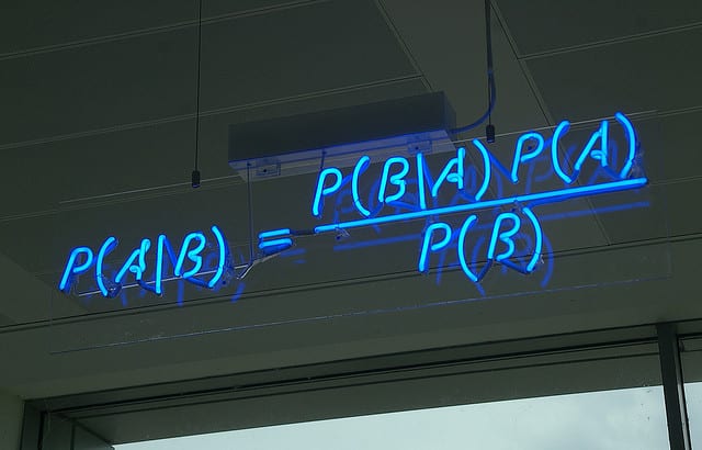
Naive Bayes Classifier

Overview:

Naïve Bayes classification is a straightforward and powerful algorithm for the classification task. Naïve Bayes classification is based on applying Bayes’ theorem with strong independence assumption between the features. Naïve Bayes classification produces good results when we use it for textual data analysis such as Natural Language Processing.

Naïve Bayes models are also known as simple Bayes or independent Bayes. All these names refer to the application of Bayes’ theorem in the classifier’s decision rule. Naïve Bayes classifier applies the Bayes’ theorem in practice. This classifier brings the power of Bayes’ theorem to machine learning.

Naive Bayes algorithm intuition:

Naïve Bayes Classifier uses the Bayes’ theorem to predict membership probabilities for each class such as the probability that given record or data point belongs to a particular class. The class with the highest probability is considered as the most likely class. This is also known as the Maximum A Posteriori (MAP).

The MAP for a hypothesis with 2 events A and B is

MAP (A)
= max (P (A | B))
= max (P (B | A) * P (A))/P (B)
= max (P (B | A) * P (A))

Here, P (B) is evidence probability. It is used to normalize the result. It remains the same, So, removing it would not affect the result.
Naïve Bayes Classifier assumes that all the features are unrelated to each other. Presence or absence of a feature does not influence the presence or absence of any other feature.

In real world datasets, we test a hypothesis given multiple evidence on features. So, the calculations become quite complicated. To simplify the work, the feature independence approach is used to uncouple multiple evidence and treat each as an independent one.

Types of Naïve Bayes algorithm:

The 3 types are listed below:-

• Gaussian Naïve Bayes
• Multinomial Naïve Bayes
• Bernoulli Naïve Bayes

Applications of Naive Bayes:

Naïve Bayes is one of the most straightforward and fast classification algorithm. It is very well suited for large volume of data. It is successfully used in various applications such as :

• Spam filtering
• Text classification
• Sentiment analysis
• Recommender systems

Dataset:

Adult Dataset

Implementation:

Libraries: NumPy pandas matplotlib sklearn seaborn

Data Exploration:

The categorical variables are :

['workclass', 'education', 'marital_status', 'occupation', 'relationship', 'race', 'sex', 'native_country', 'income']

Cardinality:

The number of labels within a categorical variable is known as cardinality. A high number of labels within a variable is known as high cardinality. High cardinality may pose some serious problems in the machine learning model.

for var in categorical:
    print(var, ' contains ', len(df[var].unique()), ' labels')

workclass  contains  9  labels
education  contains  16  labels
marital_status  contains  7  labels
occupation  contains  15  labels
relationship  contains  6  labels
race  contains  5  labels
sex  contains  2  labels
native_country  contains  42  labels
income  contains  2  labels

There are 6 numerical variables

['age', 'fnlwgt', 'education_num', 'capital_gain', 'capital_loss', 'hours_per_week']

Model training, Evaluations and Predictions:

from sklearn.naive_bayes import GaussianNB
# instantiate the model
gnb = GaussianNB()
# fit the model
gnb.fit(X_train, y_train)

Accuracy:

Training set score: 0.8067
Test set score: 0.8083
Null accuracy score: 0.7582

We can see that our model accuracy score is 0.8083 but null accuracy score is 0.7582. So, we can conclude that our Gaussian Naive Bayes Classification model is doing a very good job in predicting the class labels.

Confusion Matrix:

Classification Report:

 precision    recall  f1-score   support

       <=50K       0.93      0.81      0.86      7407
        >50K       0.57      0.80      0.67      2362

    accuracy                           0.81      9769
   macro avg       0.75      0.81      0.77      9769
weighted avg       0.84      0.81      0.82      9769

Classification Accuracy:

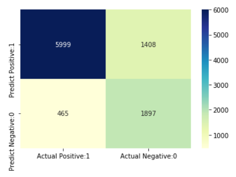
classification_accuracy = (TP + TN) / float(TP + TN + FP + FN)
Classification accuracy : 0.8083

Classification Error:

classification_error = (FP + FN) / float(TP + TN + FP + FN)
Classification error : 0.1917

Precision:

Precision can be defined as the percentage of correctly predicted positive outcomes out of all the predicted positive outcomes. It can be given as the ratio of true positives (TP) to the sum of true and false positives (TP + FP).

So, Precision identifies the proportion of correctly predicted positive outcome. It is more concerned with the positive class than the negative class.

Mathematically, precision can be defined as the ratio of TP to (TP + FP).

precision = TP / float(TP + FP)
Precision : 0.8099

Recall/ True Positive Rate:

Recall can be defined as the percentage of correctly predicted positive outcomes out of all the actual positive outcomes. It can be given as the ratio of true positives (TP) to the sum of true positives and false negatives (TP + FN). Recall is also called Sensitivity.

Recall identifies the proportion of correctly predicted actual positives.

Mathematically, recall can be given as the ratio of TP to (TP + FN).

recall = TP / float(TP + FN)
Recall or Sensitivity : 0.9281

False Positive Rate:

false_positive_rate = FP / float(FP + TN)
False Positive Rate : 0.4260

Specificity:

specificity = TN / (TN + FP)
Specificity : 0.5740

Calculate class probabilities:

We can rank the observations by probability of whether a person makes less than or equal to 50K or more than 50K.

y_pred_prob = gnb.predict_proba(X_test)[0:10]

array([[9.99999426e-01, 5.74152436e-07],
       [9.99687907e-01, 3.12093456e-04],
       [1.54405602e-01, 8.45594398e-01],
       [1.73624321e-04, 9.99826376e-01],
       [8.20121011e-09, 9.99999992e-01],
       [8.76844580e-01, 1.23155420e-01],
       [9.99999927e-01, 7.32876705e-08],
       [9.99993460e-01, 6.53998797e-06],
       [9.87738143e-01, 1.22618575e-02],
       [9.99999996e-01, 4.01886317e-09]])

Observations:

• We can see that the above histogram is highly positive skewed.
• The first column tell us that there are approximately 5700 observations with probability between 0.0 and 0.1 whose salary is <=50K.
• There are relatively small number of observations with probability > 0.5.
• So, these small number of observations predict that the salaries will be >50K.
• Majority of observations predcit that the salaries will be <=50K.

ROC-AUC:

ROC AUC stands for Receiver Operating Characteristic - Area Under Curve. It is a technique to compare classifier performance. In this technique, we measure the area under the curve (AUC). A perfect classifier will have a ROC AUC equal to 1, whereas a purely random classifier will have a ROC AUC equal to 0.5.

ROC AUC : 0.8941

K-Fold cross validation:

from sklearn.model_selection import cross_val_score
scores = cross_val_score(gnb, X_train, y_train, cv = 10, scoring='accuracy')
print('Cross-validation scores:{}'.format(scores))

Cross-validation scores:[0.81359649 0.80438596 0.81184211 0.80517771 0.79640193 0.79684072
 0.81044318 0.81175954 0.80210619 0.81035996]

Learnings:

Feature endineering Feature Scaling Cardinality

References:

Naïve Bayes and Bernoulli Naïve Bayes

Feedback

If you have any feedback, please reach out at pradnyapatil671@gmail.com

🚀 About Me

Hi, I'm Pradnya! 👋

I am an AI Enthusiast and Data science & ML practitioner