Turbulence Driver
The turbulence driver will generate velocity perturbation in the Fourier space and add to the velocity field by taking the inverse FFT.
There are three types of driving controlled by the parameter turb_flag (must be set in the input file under the <problem> block):
-
turb_flag=1: perturbation is only added at the beginning of the simulation (decaying turbulence).dedtin this case sets the total kinetic energy. -
turb_flag=2: perturbation is added with an interval set by a user bydtdrive(impulsive driving). -
turb_flag=3: perturbation is added continuously with an interval of the simulation time stepdt(continuous driving).
Some parameters for turbulence driving/initialization need to be set in the input file under the <turbulence> block (see inputs/hydro/athinput.turb):
-
dedt: energy injection rate (for driven) or total energy (for decaying) -
nlow: cut-off wavenumber at low-k -
nhigh: cut-off wavenumber at high-k -
expo: power-law exponent of the power spectrum (P_v ~ k^{-expo}) -
tcorr: correlation time for the OU process (both impulsive and continuous) -
dtdrive: time interval between perturbation (impulsive) -
f_shear: the ratio of the shear component -
rseed: seed for the random number. If negative, the seed will be automatically set. If non-negative, the seed will be set by hand (not recommended forturb_flag=3; see below)
The power spectrum of velocity perturbation follows a power law within the wavenumber range between nlow and nhigh with an exponent set by expo parameter. For a given random number seed rseed, each velocity component is realized by a Gaussian random field. The velocity perturbation is decomposed into solenoidal and compressive components and added with a ratio set by f_shear. For example, if f_shear=0, turbulence driving is fully compressive, and if f_shear=1, turbulence driving is fully solenoidal.
For driven turbulence (turb_flag=2 and 3), dedt denotes the energy injection rate so that the total kinetic energy injected at every driving step is dedtxdtdrive for turb_flag=2 and dedtxdt for turb_flag=3. We adopt the Ornstein-Uhlenbeck process to smoothly change perturbations over the correlation time tcorr.
> ./configure.py --prob=turb -fft
> ./athena -i ../inputs/hydro/athinput.turb problem/turb_flag=[1,2,3]
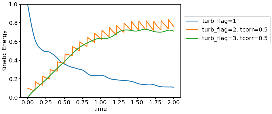
The time evolution of kinetic energy for different turb_flag (f_shear=0.5, dtdrive=0.1, tcorr=0.5):
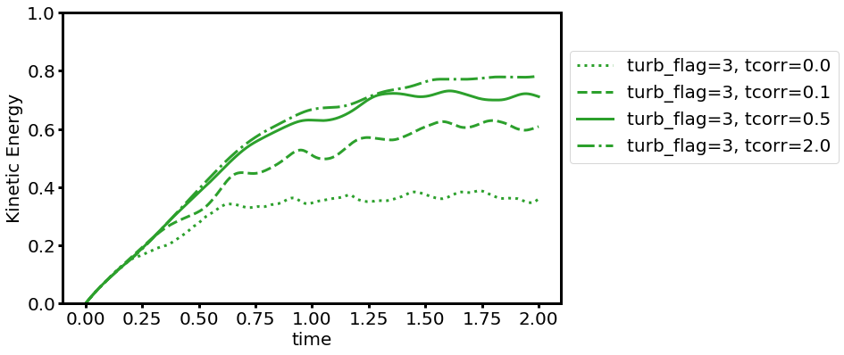
The time evolution of kinetic energy for different tcorr (turb_flag=3, f_shear=0.5):
For a non-negative rseed, an identical random number sequence is guaranteed for the same domain setup. However, this procedure makes the generation of power spectrum slow. Therefore, there will be a serious performance hit if rseed>=0 and turb_flag=3.
If performance is an issue and if your problem type is fine with using only a few modes for the driving, @pgrete implemented a version of the driving where the "global" inverse transform is done on each MeshBlock separately (manually and not using an external library) and no communication (expect a single scalar for normalizing) is required between the blocks. This works fine if only a few modes are excited, e.g., the total overhead of the driving is about 30% of an MHD step when using about 30 modes IIRC. More details (on the effectively identical implementation in K-Athena) can be found here: https://gitlab.com/pgrete/kathena/-/wikis/turbulence