Fourier-Hankel implementation for direct and inverse Abel transforms

[rth]

Probably won't be too hard to implement at some point, if somebody is interested. See FHA cycle

The only thing that need to be cheked is whether the Hankel transform can be done exclusively with numpy, scipy (don't know if scipy.linalg.hankel is related) or whether we would need to use a separate package hankel.

In which case it can be added as an optional dependency, and this implementation should raise an error if hankel module is not installed (trying to keep the number of additional dependencies low). Or any other way you prefer to handle this.

[DanHickstein]

Yes, it would be fun to include the FH version of the transform for comparison purposes!

The scipy.linalg.hankel says that it constructs a "Hankel Matrix". Wikipedia says that the Hankel Transform is "Not to be confused with the determinant of the Hankel matrix of a sequence."

So, I think that we may need to use that package that you suggest, or figure something else out.

[DanHickstein]

This should be pretty easy to implement, but, when I looked around the literature, I could not find a clear equation for the Fourier-Hankel transform, despite it being mentioned frequently. @stggh, do you know of a paper that gives the equation/algorithm for the FH transform?

[stggh]

Python code for the Hankel transform is available at this github.

The HankelTransform function requires a function (image) input rather than (grid) data. At the moment I am confused by the evaluation of the Hankel transform in radial (1D) space, and how to return the 2D image, although, the (slightly buggy) examples appear to cover this case.

Thoughts, suggestions?

[DanHickstein]

Oh, that is pretty cool that you found code for the Hankel transform. It looks like that code is just for the 1D case, right? We would just need to loop over all rows (or, hopefully, vectorize somehow).

It looks like that package was developed reasonably recently, so the author might be able to help us wrangle it into a Fourier-Hankel transform function.

[stggh]

@DanHickstein my apologies for the delay in my response. My coding time is limited at the moment, due to an upcoming teaching semester. @steven-murray author of the hankel is very helpful. I just have not had time to work through the 2D implementation, but will do so, once I have some free time.

[steven-murray]

Hi there,

Would love to figure out how to get hankel to do what you need it to do. It currently just does the 1D Hankel transform -- which covers any n-dimensional radially symmetric Fourier transform.

Having briefly read through this thread -- it seems like you need a 2D image. My code will of course do this fine if the image is radially symmetric. I have never considered a case where there is not radial symmetry (radial symmetry is usually the reason you'd use a hankel transform in the context of a FT). Just let me know what you need and I should be able to help out pretty easily.

Cheers.

[stggh]

Velocity-map images are (at least) "radially" symmetric in 1-d, about axis=0, along each image row.
e.g. O^-₂ photoelectron image:

It would be preferable not to have to iterate row-by-row.

[steven-murray]

Hmmm, so is a 2D FT required, or a 1D FT over each row?

[DanHickstein]

@steven-murray, Thanks for being willing to help us out!

Everything happens in 1D. And, conceptually, each row can be treated separately.

When @stggh says that we want to avoid iterating "row-by-row", he is pointing that, to achieve the highest efficiency, we need to avoid for loops in Python, and instead vectorize our calculations using 2D numpy arrays. (So, there are still for loops, but they are just getting done by the c-code in numpy).

Anyway, for a proof-of-principle demonstration, it's totally fine to iterate over the rows in Python, as far as I am concerned. We can figure out how to speed things up after we get reasonable results.

Big picture: the "Fourier-Hankel" transform is mentioned in many papers about Abel transform as something of the "1980's gold standard" that has now been improved upon. We always thought that PyAbel should include it, because everyone talks about it so much, but we never really knew a good implementation of the Hankel transform, and I'm not sure that I ever really found a paper that explains how this "Fourier-Hankel" transform should be completed.

This thesis seems to say that we just need to take an inverse Hankel transform of the FT of our data:

http://trace.tennessee.edu/cgi/viewcontent.cgi?article=4324&context=utk_gradthes

I am curious to see how the FH transform compares with the other methods. It may offer a different efficiency scaling with the image size, and may be able to handle larger images. And it may offer an advantage in that it doesn't need to pre-compute and basis-sets like many of the other transform methods.

[stggh]

I agree our main aim is to implement the F-H transform (and if possible improve the execution speed), and Eq. (2.7) appears correct, according to @rth's FHA cycle top comment:

FA = H, hence A^-1 F^-1= H^-1, and therefore A^-1 = H^-1F

As @DanHickstein states, we process each row, Fourier transform and then inverse Hankel transform.

[steven-murray]

Okay cool. Well, hankel doesn't do a discrete transform as its primary goal (not in the same way that say a DFT is a discrete transform which can be written as a matrix equation). It's main purpose is to perform an accurate Hankel integral, which provides for an accurate transform for a given k. It can vectorize this operation for a vector of k, but this won't be quite as fast as a simple discrete transform (or any of the more efficient versions introduced in that thesis).

This is why hankel is written to accept a callable function f(x) to integrate/transform.

I'm wondering if there's a reason you don't want to use the basic "Direct HT" given in Eq. 2.12 of the thesis you shared? It would be easy to implement, easy to vectorize, and probably faster than hankel for your problem.

I'm assuming that you start the problem only with a discrete 2D array, not an analytic function?

[stggh]

hankel doesn't do a discrete transform

Bummer! Sorry, that I did not realise this.

use the basic "Direct HT" given in Eq. 2.12

Path of least pain ;-) Eq. 2.12 requires a little thought.

[steven-murray]

I have been thinking about implementing some discrete HT functions in hankel, so they might appear soon.

I should clarify my last comment -- hankel will do a discrete transform if you force it to, it's just not built to do it. The way to do it is to use a spline on your array. The biggest problem is that it uses the same underlying array for each k, which has N elements (N is a parameter to hankel, not the length of the input function). Due to the way it's built, this array underlying the transform has to be good enough to get the integral right for all k in the vector you pass, which basically means the worst one sets the performance level. If you have a big dynamic range, this can be a killer. If not, then you're ok, and hankel will perform alright (similar to a direct HT, except more accurate).

Here's a small implementation of the DHT that I just wrote (it seems to work on a simple Gaussian function):

from scipy.special import jn
import numpy as np
from numpy.fft import fft, hfft, fftfreq, fftshift

def construct_dht_matrix(N, nu  = 0, b = 1):
    m = np.arange(0,N).astype('float')
    n = np.arange(0,N).astype('float')
    return b * jn(nu, np.outer(b*m, n/N))

def dht(X, d = 1, nu = 0, axis=-1, b = 1):
    N = X.shape[axis]
    
    prefac = d**2
    m = np.arange(0,N)
    freq = m/(float(d)*N)
    
    F = construct_dht_matrix(N,nu,b)*m
    return prefac * np.tensordot(F,X, axes=([1],[axis])), freq

This works for arbitrary dimension matrix X. Setting b sets the frequency normalisation (the thesis uses b=2pi). It's pretty quick as well.

I tried also writing the Abell transform, as specified by Eq. 2.13 in the thesis. I'm getting something slightly wrong (probably the frequency normalisation), but the code I have thus far is

def hankel_fourier_transform(X, d=1, nu = 0):
    N = X.shape[-1] # Assuming we're doing transform on second axis (X is 2D here)
    
    # Assumes X is 2D and has symmetry about 0
    G = np.real(fftshift(fft(X, axis=-1))[:,N/2:]*d) # Just get non-negative frequencies
    
    # Now the DHT
    eps = dht(G, d=1/(N*d), nu=nu, b=np.pi)[0] * 2  #b=pi to account for N/2, then *2 to get 2pi out front
    
    return eps, d*np.arange(0,N/2)

Feel free to play around with these. Doing this has sparked some ideas for things to implement in hankel, so it might get an update soon ;-)

[stggh]

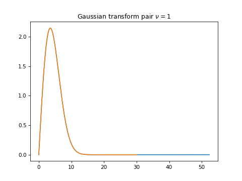
@steven-murray fantastic - great work!

I can confirm the Gaussian discrete Hankel transform, although I am also not sure about the normalization.

code here

For the inverse Abel transform we pass 1/2 image row (right-side), a 1d-numpy array. This may then duplicated for the (r)fft np.append(X[::-1], X), followed by the dht on G. Repeat for each row.

Testing this for inverse Abel transform

[stggh]

Some progress, but the profile is overcorrected.

very poor coding here

[steven-murray]

Thanks @stggh , this looks promising -- certainly using the zeros of the Bessel function is more akin to the way that hankel works. Making this a proper DHT will be very useful.

I don't have much time this week as I am away for a conference, but will plug away at it when I can.

[steven-murray]

Neat! Amazing sympy? ;-)

Actually, this time I just used Wolfram|Alpha on each term separately :-)

[stggh]

The "secret" is to sample the function correctly:

---

This then yields Fig 1.(a), (c), for the Gaussian trial function 'forward' Hankel transform:

poor quality code gist for the above figure

[stggh]

The "trick" for the Hankel transform is that the source function is evaluated at the spherical Bessel function zeros. A radial range r = 0, ..., n-1 becomes jz*(n-1)/jz[N] where jz = scipy.special.jn_zeros(nu, N+1) and N is chosen so that jz[N] ~ n-1. jz then selects the sample points.

More later, at this moment I am also time poor.

[stggh]

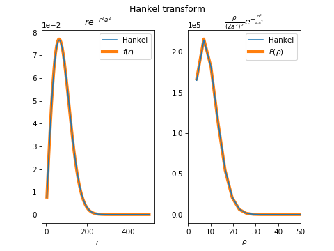
This code gist appears to correctly (forward, inverse) transform the Baddour analytical exponential transform pairs. This image shows the numerical transform with its analytical function:

The only issue appears to be the need to sample our PyAbel images on to the Bessel grid

[stggh]

Improved version of the transformation_matrix:

def transformation_matrix(jz, nu=0):
    # Baddour transformation matrix Eq. (25) JOSA A32, 611-622 (2015)
    b = 2/(jn(nu+1, jz) * jn(nu+1, jz) * jz[-1])

    return b * jn(nu, np.outer(jz, jz / jz[-1]))

Updated code gist

[steven-murray]

This all looks really good. It is frustrating that a re-sampling has to be performed, It would be nice to be able to directly use an input discrete array.

I'm trying to think of a way around this, but can't at this point (my own hankel code also uses the Bessel zeros as nodes of the integration, so this seems to be a common theme amongst discrete Hankel transform methods).

We could perhaps build a reasonably robust case-by-case system in which an input array is interpolated onto the correct grid. It would be hard to vectorize well though, and interpolation always turns up problems for bad functions.

I might give it a shot this afternoon, and add a few tests in as well.

[stggh]

I find the sample space selection confusing. I think the required sampling condition is in fact the product space x frequency = jn_zeros(nu, N+1) i.e. choose N so that r_max x ρ_max ~jz[N].

This gist is the Baddour sinc function test, Eq.s (84, 85). The above condition gives N=286, similar to the selected 256 in Baddour's paper:

@steven-murray thanks for keeping a tag on this. I am sure you understand much more about these transform sample spaces that I do. I agree, interpolation of each image row intensity will be necessary, but perhaps there is some clever @DanHickstein map_coordinates() function that may be applied to the image.

[stggh]

Image interpolation is not a good idea because of the measurement noise. We may as well return to the discrete version of the basic definition:

and @steven-murray original code above, which, I think(?), is the a fast version of Whittaker C-code Imaging in Chemical Dynamics, that I converted to Python (below). This Hankel transform operates on each image row, without requiring interpolation.

def Hankel(F, nu=0):
    """
    Whitaker "Image reconstruction: the Abel transform" Ch 5

    Parameters
    ----------
    F : numpy 1D array
       image row
  
    Returns
    -------
    f : numpy 1D array
       Hankel transform
    """

    n = F.size

    Nyquist = 1/(2*n)

    f = np.zeros_like(F)
    for i in range(n):
       for j in range(n):
           q = Nyquist*j
           f[i] += q*F[j]*jn(nu, 2*np.pi*q*i)

    return f

I will play some more. Sorry, for the diversion into the Baddour algorithm, which appears more suitable for analytical functions.

[stggh]

Vectorized Whitaker code:

    n = F.size

    Nyquist = 1/(2*n)

    f = np.zeros_like(F)
    i = np.arange(n)

    for j in range(n):
       q = Nyquist*j
       f[:] += q*F[j]*jn(nu, 2*np.pi*q*i[:])

    return f

code gist

Not sure about frequency axis or amplitude scaling. @steven-murray I have not reconciled your original code (edit: code is fine). Out of free time at this moment.

[stggh]

Here is the sinc function transform pair:

code gist

[stggh]

The @steven-murray version of the Hankel transform is good, equivalent to, but faster than, Whitaker's and they both pass the Baddour analytical function (Gaussian, Sinc) transform pair test. The issue of the Fourier-Hankel transform of curve A (above) remains.

[stggh]

discrete Fourier transform

Sorry for the (testing noise). I think we are getting close.

A check of the dft function for a square pulse, which should give a sinc function, shows that every second rfft element is zero. Hence, only the even elements of the rfft array must be selected, but his means that the return array is only 1/2 size. I am missing a detail?

code gist

[DanHickstein]

It looks like @stggh is very close to a working FH transform. So, probably this isn't especially relevant, but, for the record, I found a matlab implementation of the FH transform hiding in the original BASEX matlab code: https://github.com/PyAbel/PyAbelLegacy/blob/master/BASEX/Matlab/fourier_hankel.m

[steven-murray]

with 8f6b0bb has this all been solved? I have been away from this for a while, and returned to it for half a day before I went on vacation. What is the current state of play?

[steven-murray]

I think it would be good (for me at least) to write this up with several analytical tests to make sure it works in various situations. On my own testing, I've found that the normalisation issue we encountered previously in the Gaussian case is due to resolution/finite range. This means the algorithm is correct, but it just needs to be used with care (i.e. it's the user's problem!). It would be good to have a jupyter notebook or something like that to be able to easily run through and see how it's used, where it works and where it doesn't.

[stggh]

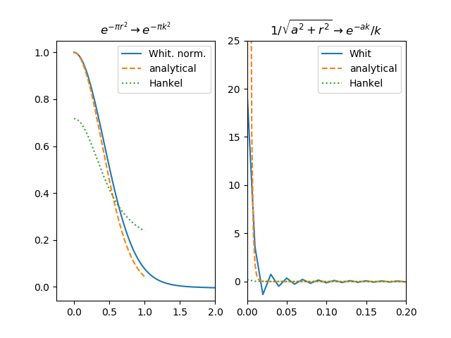
Not solved. I left this problem, meaning to come back to it, but I was diverted.

Your synopsis is right.

due to resolution/finite range

I have spent a lot of time going around in circles due to the spatial/frequency domain issues, and sampling.

I am not convinced that your/Baddour like algorithm, without Bessel zero sampling, is correct, but perhaps, I have stuffed the implementation along the way (highly likely).

Here are 2 transform pairs that get mangled, the right side is a sampling issue:

How would you like to proceed? The hankel-basic.py above has both my version of the Whitaker code and yours, for the sinc transform pair. Is this of any use?

[stggh]

Here is the corresponding jupyter notebook

[stggh]

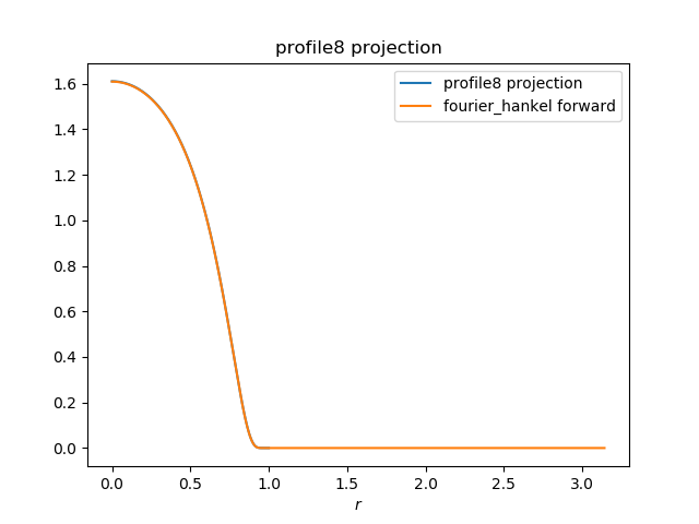
fourier_hankel forward transform appears to be working:

The tricky part is the grid corresponds to π r, which may necessitate interpolation to return to the image grid (?).

plot code gist using fourier_hankel.py of my PyAbel fork fourier_hankel branch.

Playing with inverse transform now ...

[stggh]

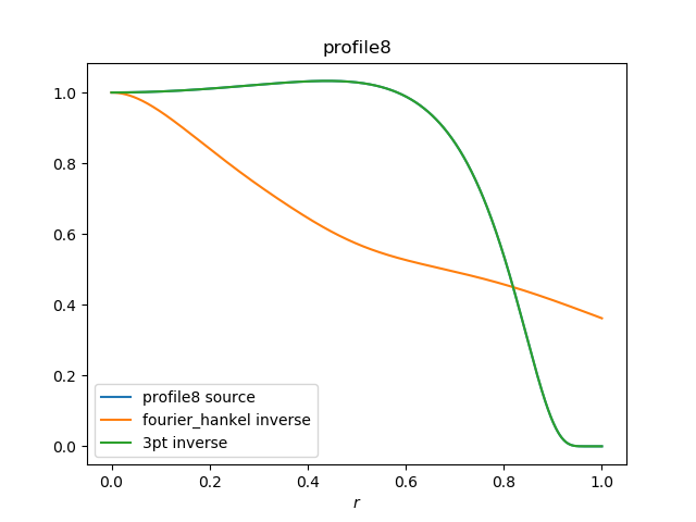
So, no problem with the @steven-murray clever code for the fourier_hankel forward Abel transform:

The inverse Abel transform fails:

Key code fourier_hankel.py, also available on my fourier_hankel branch:

def dht(X, dr=1, nu=0, axis=-1, b=1):
    # discrete Hankel transform
    N = X.shape[axis]

    n = np.arange(N)

    freq = n/dr/N

    F = b * jn(nu, np.outer(b*n, n/N)) * n

    return dr**2 * np.tensordot(X, F, axes=([1], [axis])), freq


def dft(X, dr=1, axis=-1):
    # discrete Fourier transform

    # Build a slicer to remove last element from flipped array
    slc = [slice(None)] * len(X.shape)
    slc[axis] = slice(None, -1)

    X = np.append(np.flip(X, axis)[slc], X, axis=axis)  # make symmetric

    fftX = np.abs(np.fft.rfft(X, axis=axis)) * dr
    freq = np.fft.rfftfreq(X.shape[axis], d=dr)

    return fftX, freq


def fourier_hankel_transform(IM, dr=1, direction='inverse',
                             basis_dir=None, nu=0, axis=-1):
    IM = np.atleast_2d(IM)

    if direction == 'inverse':
        fftIM, freq = dft(IM, dr=dr, axis=axis)  # Fourier transform
        # Hankel
        transform_IM, freq = dht(fftIM, dr=freq[1]-freq[0], nu=nu, axis=axis)
    else:
        htIM, freq = dht(IM, dr=dr, nu=nu, axis=axis)  # Hankel
        transform_IM, freq = dft(htIM, dr=freq[1]-freq[0])  # fft
        freq *= 2*np.pi   

    if transform_IM.shape[0] == 1:
        transform_IM = transform_IM[0]   # flatten to a vector

    return transform_IM, freq

Note, this function returns "image" and frequency, unlike the usual PyAbel transforms.

I have a feeling that I am missing something obvious for the direction="inverse" code ...

(Edit: fix code copy error)

[steven-murray]

this looks good! Sorry I haven't had enough time to do anything on this recently. Is there a normalisation problem with the inverse?

[gauteh]

A good resource with many references on the FHT (or the FFP) is chapter 4 Wavenumber Integration Techniques in Computational Ocean Acoustics (usually available through university accounts). E.g.: chapter 4.5.6.

[DanHickstein]

Hi @gauteh, thanks for pointing this out!

When you write FHT, I originally thought that you were referring to the "Fourier Hankel Transform", but now that I have looked up the book chapter, I see that FHT = "Fast Hankel Transform".

I believe that @stggh and @steven-murray have some numerical version of the Hankel transform working already. But, probably the references in that book contain more efficient algorithms for the Hankel Transform, which could speed things up.

[gauteh]

Danhickstein writes on februar 19, 2018 18:00:

Hi @gauteh, thanks for pointing this out! When you write FHT, I originally thought that you were referring to the "_Fourier_ Hankel Transform", but now that I have looked up the book chapter, I see that FHT = "_Fast_ Hankel Transform". I believe that @stggh and @steven-murray have some numerical version of the Hankel transform working already. But, probably the references in that book contain more efficient algorithms for the Hankel Transform, which could speed things up.

Worth checking out at least! I have not looked in detail on the difference with the implementations here. Both the Fast Field Approximation and Fast Hankel Transform as described in this reference use the asymptotic versions of the Hankel functions. But the version of the Fast Hankel Transform (which does not seem to uniquely refer to one method) can use the full Bessel functions for lower wavenumbers*ranges as well as the negative spectrum as well.