20337143 杨锐佳 中山大学 计算机科学与技术
sb981335043/RL_DQN (github.com) GITHUB repository

In a Breakout game:
-
A player is given a paddle that it can move horizontally
-
At the beginning of each turn, a ball drops down automatically from somewhere in the screen*
-
The paddle can be used to bounce back the ball
-
There are layers of bricks in the upper part of the screen
-
The player is awarded to destroy as many bricks as possible by hitting the bricks with the bouncy ball
-
The player is given 5 turns in each game
In this mid-term project, you will be given a full implementation of a Nature-DQN agent, and the assignments include: Team up with another one registered in this course Read through the implementation and explain in detail in your team report what each component is responsible for and how the components are connected together Pick one of the questions below that you together with your teammate should research into:
- Can you boost the training speed using Prioritized Experience Replay?
- Can you improve the performance (e.g., using Double DQN or Dueling DQN)?
- Can you stabilize the movement of the paddle (avoid high-freq paddle shaking effects) so that the agent plays more like a human player?
- Can you accelerate the training speed (e.g., using Asynchronous Advantage Actor-Critic)? (See more in the next slide)
Explain your work and exhibit the performance gain (or explain why things won’t work) in your team report
-
Important: all enhancements should base on the given implementation
-
Bonus 1: Analyze the theoretical and physical significance of the performance-enhancing tricks you add in detail
-
Bonus 2: Open-source your project on GitHub, Gitee, or any other similar platforms and include a reference link in your team report
-
Bonus 3: Compose your report in English

Q-learning is a very important off-policy learning method in reinforcement learning, which uses Q-Table to store the value of each state action pair, while it is not practical to use Q-Table when the state and action space is high-dimensional or continuous.
Therefore, the Q-Table update problem is turned into a function fitting problem, and a neural network is used to obtain the Q-value of the state action, and the Q-function is made to approximate the optimal Q-value by updating the parameter θ , which is the basic idea of DQN.
However, the combination of deep neural networks and reinforcement learning ideas inevitably lead to some problems, such as: 1、DL requires a large number of samples with labels for supervised learning; RL requires only reward return values. 2、the samples of DL are independent; the states before and after RL are related 3、DL target distribution is fixed; the distribution of RL keeps changing, for example, if you play a game, the distribution of states in one level and the next level is different, so after training the previous level, the next level has to be retrained again. 4、Previous research has shown that problems such as instability arise when using nonlinear networks to represent value functions.
To solve Problem 1, we have to use the Bellman equation.


The two equations above, the first is the Bellman expectation equation and the second is the Bellman optimality equation. In our actual problems, for one state, a specific action is taken and the next state is essentially determined,So we can remove the summation from the optimal equation. In this way,we can get a prediction of the Q value by the neural network,and a target value of Q is obtained by Bellman's optimal equation, and supervised learning is performed by the gap between the predicted value and the target value.
To solve problems 2 and 3, we use the Experience Replay method by storing the transfer samples (st,at,rt,st+1,is_terminal) obtained from the interaction between the agent and the environment at each time step in the experience pool and taking out some random (minibatch) when we want to train. This avoids the correlation problem.
We can explain question 4 once again.According to the above idea, we need the network to get the Q-prediction of the current state action, and also need to get the Q-prediction of the state-optimal action at the next moment through the network, and then get the Q-target value of the current state action through the Bellman equation, and update the network parameters according to the Q-target value and the Q-prediction.It's like a self-directed movie, or a contest where you are both a player and a referee, making the network very unstable.To solve this problem, we propose a dual network structure.In this way, the Q prediction is obtained from the eval-net, while the Q target value is obtained based on the current immediate reward r and the target-net.
Therefore, the final loss function in DQN is as follows:

In the above equation, θ denotes the parameters of eval-net, while θ across denotes the parameters of target-net. In practical applications, the parameters of target-net are copied from eval-net at regular intervals.

In the experience pool of traditional DQN, the data of batch is selected for training is uniformly distributed randomly, without considering the priority relationship of samples. But in fact, the value of different samples is different, and we need to give each sample a priority and sample according to the priority of the sample.
How are samples prioritized? We can use TD-error, which means q-target - q-eval, to specify the priority of learning. The larger the TD-error is, the more room we have for improvement in prediction accuracy, and the higher the sample needs to be learned, the higher the priority p is.
With TD-error, we have a priority p, but how do we sample efficiently according to p? It would be very computationally intensive to sort all samples by p for each sampling. A method called SumTree has been proposed.
SumTree is a tree structure, the leaf node stores the priority p of each sample, each branch node has only two forks, and the value of the node is the sum of the two forks, so the top of SumTree is the sum of all p. As shown in the figure below: the bottom layer of leaves stores the p of samples, the leftmost 13 = 3 + 10 in the upper layer of leaves, and the root of the top layer is the sum of all p according to this rule.

When sampling, we divide the sum of p by the batch size into as many intervals as the batch size, (n=sum(p)/batch_size). If we add up the priority of all nodes to 42, then if we draw 6 samples, the priority of the interval at that time may be like this:
[0-7], [7-14], [14-21], [21-28], [28-35], [35-42]
Then pick a random number in each interval. For example, if we pick 24 in the interval [21-28], we will search down from the top 42 according to this 24. First, we see that there are two children nodes below the top 42, so we take the 24 in our hand and compare the left child node, because 29>24, then we will take the left path; then we compare the left child node 13 of 29, because 24>13, then we will take the right path, and modify the value in our hand according to 13, to 24-13 = 11. Then we take 11 and compare the left child node 12 of 13, and the result is 12 is larger than 11, then we will choose 12 corresponding to as the result of sampling this interval.
In the original DQN, there may be cases where the Q estimate is higher because we use an off-policy policy, where instead of using the real action used in the next interaction, we take the action that the current policy thinks has the highest value each time we learn, so there is an overestimate of the Q value.And in DQN, we face the same problem because we use target-net when choosing the next moment action and when calculating the next moment state-action Q value.
In order to decouple action selection and value estimation, we have the Double-DQN method. In Double-DQN, in calculating the actual value of Q, the action selection is obtained from eval-net, and the value estimation is obtained from target-net. At this point, the loss function becomes.

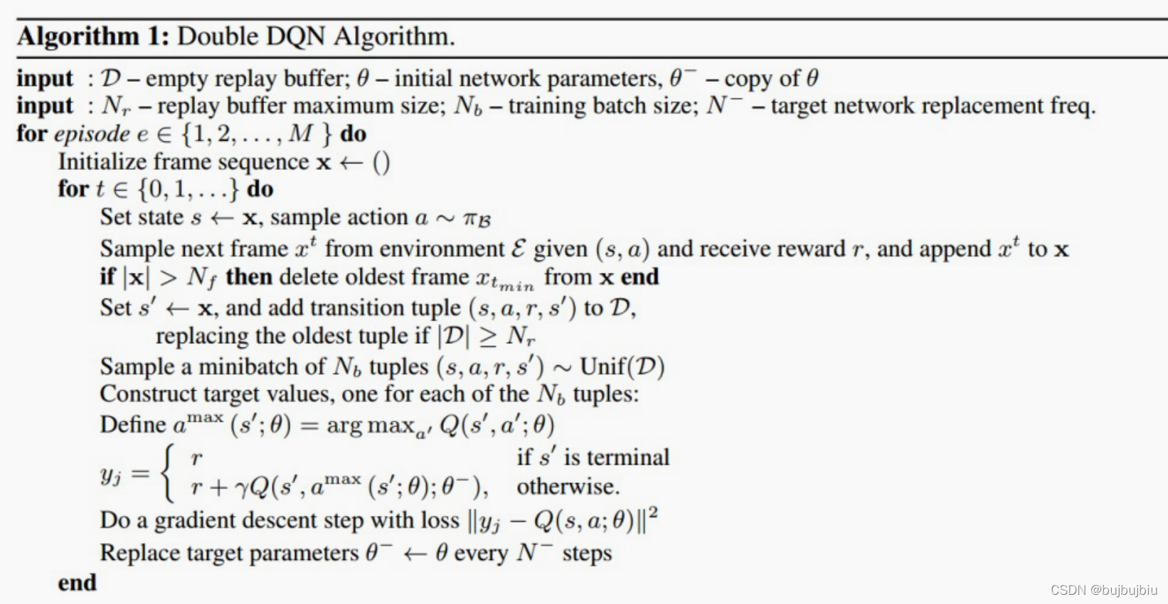
Since Double Q-learning requires the construction of two action value functions, one for estimating the action and another for estimating the value of that action. Considering that two networks, evaluation network and target network, are already available in the DQN algorithm, the DDQN algorithm only needs to use the evaluation network to determine the action and the target network to determine the action value when estimating the return, without constructing a new network separately. Therefore, we only need to change the method of calculating the target value in the DQN algorithm as follows:
Here is the equation after the change:
The algorithm process of DDQN algorithm and Nature DQN is exactly the same except for the way the target Q value is calculated. Here we summarize the algorithmic flow of DDQN.
Algorithm inputs: number of iteration rounds T, state feature dimension n, action set A, step size α, decay factor γ, exploration rate ϵ, current Q-network Q, target Q-network Q′, number of samples m for batch gradient descent, target Q-network parameter update frequency C.
Algorithm output: Q network parameters
      1. Randomly initialize all states and actions corresponding to the value Q. Randomly initialize all parameters w of the current Q-network,initialize the parameters w′=w of the target Q-network Q′. Empty the set D of experience playback.

         2. for i from 1 to T,perform iterations。
a) Initialize S to be the first state of the current state sequence, and get its feature vector ϕ(S)
b) Using ϕ(S) as input in the Q-network, the Q-valued outputs corresponding to all actions of the Q-network are obtained. Select the corresponding action A in the current Q-value output using the ϵ-greedy method
c) Execute the current action A in state S,get the feature vector ϕ(S′) and reward ϕ(S′) and reward R$ corresponding to the new state S′,whether to terminate the state is_end
d) The quintet {ϕ(S),A,R,ϕ(S′),is_end}{ϕ(S),A,R,ϕ(S′),is_end} is stored in the experience playback set D
e) S=S′
f) Sampling m samples {ϕ(Sj),Aj,Rj,ϕ(S′j),is_endj},ϕ=1,2,,,m from the empirical playback set D, the current target Q value yj is calculated.

g) All parameters of the Q network are updated using the mean squared loss function by back propagation of the gradient of the neural network w
h) If i%C=1,then update the target Q-network parameter w′=w
i) If S′ is terminated, the current round of iterations is completed, otherwise go to step b)

Above is our traditional DQN, and below is our Dueling DQN. In the original DQN, the neural network directly outputs the Q value of each action, while the Q value of each action in the Dueling DQN is determined by the state value V and the dominance function A, i.e., Q = V + A.
The idea of Dueling DQN is to independently learn Value and Advantage and add them up to form Q, instead of learning all Q values directly as in traditional DQN.
What is a state value function? It can be understood as the sum of the action value function corresponding to all possible actions in that state multiplied by the probability of taking that action. In more general terms, it is the value function.
What is the dominance function? We can simply understand it as the difference between the value that can be obtained by taking an action for a particular state and the average value that can be obtained for that state. If the value of the action taken is greater than the average value, then the dominance function is positive, and vice versa.
Is it possible to simply use Q = V + A? Of course not, because for a definite Q, there are an infinite number of combinations of V and A to obtain Q. Therefore, we need to impose certain restrictions on A. Usually, the mean value of the dominance function A in the same state is restricted to 0.
Therefore, our formula for calculating Q is as follows.

- First let's implement Sumtree, which is the basis for priority experience repaly
- SumTree 的构建更新和插入 - 知乎 (zhihu.com)
- We have to complete the implementation of insert, update, propagate, extract and other operations
import numpy as np
import torch

class SumTree:

    def __init__(self , capacity, device):
        self.capacity = capacity
        self.tree = torch.zeros(2*capacity - 1).to(device)
        self.data = torch.zeros(capacity,dtype = object).to(device)
        self.n_entries = 0
        self.write = 0

    def _propagate(self , idx , change):
        parent = (idx - 1) // 2
        self.tree[parent] += change

        if parent!=0:
            self._propagate(parent , change)

    def _retrieve(self , idx , s):
        left = 2* idx + 1
        right = left + 1

        if left >= len(self.tree):
            return idx
        if s <= self.tree[left]:
            return self._retrieve(left , s)
        else:
            return self._retrieve(right , s - self.tree[left])

    def total(self):
        return self.tree[0]

    def add(self, p ,data):
        idx = self.write + self.capacity - 1
        self.data[self.write] = data
        self.update(idx, p)
        self.write += 1
        if self.write >= self.capacity:
            self.write = 0
        if self.n_entries < self.capacity:
            self.n_entries += 1

    def update(self, idx, p):
        change = p - self.tree[idx]
        self.tree[idx] = p
        self._propagate(idx, change)

    def get(self, s):
        idx = self._retrieve(0, s)
        dataIdx = idx - self.capacity + 1
        return (idx, self.tree[idx], self.data[dataIdx])
ATTENTION: Be sure to use the variable types in the Torch library to make these variables available to the GPU during training, otherwise it will result in this data running on the CPU, thus causing the model body to run on the GPU while SUMTREE runs on the CPU, which will make the CPU and bus full in the face of the great amount of data exchange, while the SWAP partition of memory is bursting at the seams and training is extremely slow!
The essential difference between priority experience playback and Baseline lies in the way we select the batch, so that we can just modify the sample() sampling function in utils_memory.py and change the random sampling to pick a random number in each interval on SUMTREE and search from the root down.
-
#根据优先值从根部向下搜索得到叶子内数据
	def get_leaf(self, v):
        parent_idx = 0
        while True:		#while for the better performance
            cl_idx = 2 * parent_idx + 1         # this leaf's left and right kids
            cr_idx = cl_idx + 1
            if cl_idx >= len(self.tree):        # reach bottom, end search
                leaf_idx = parent_idx
                break
            else:       # downward search, always search for a higher priority node
                if v <= self.tree[cl_idx]:
                    parent_idx = cl_idx
                else:
                    v -= self.tree[cl_idx]
                    parent_idx = cr_idx

        data_idx = leaf_idx - self.__capacity + 1
        return leaf_idx, data_idx		#return the leaf_id and data
-
And the implementation of
sample()reads as follows -
    def sample(self, batch_size: int) :
        #actions, rewards , dones =  [], [], []
        idxs = torch.zeros((batch_size), dtype=torch.long).to(self.__device)
        indices = torch.zeros((batch_size), dtype=torch.long).to(self.__device)
        segment = self.total_p() / batch_size

        #-----------------HERE IS THE ADDITION------------------------
        #改随机取样为利用SumTree分段随机抽取
        for i in range(batch_size):
            a = segment*i
            b = segment*(i+1)
            s = random.uniform(a,b)
            idx , dataidx =self.get_leaf(s)

            idxs[i] = idx
            indices[i] =dataidx
        #-------------------------HERE------------------------

        b_state = self.__m_states[indices, :4].to(self.__device).float()
        b_next = self.__m_states[indices, 1:].to(self.__device).float()
        b_action = self.__m_actions[indices].to(self.__device)
        b_reward = self.__m_rewards[indices].to(self.__device).float()
        b_done = self.__m_dones[indices].to(self.__device).float()

        return idxs, b_state, b_action, b_reward, b_next, b_done
- 所谓的Double Q Learning是将动作的选择和动作的评估分别用不同的值函数来实现。
    def prior_learn(self, memory: ReplayMemory, batch_size: int) -> float:
        """learn trains the value network via TD-learning."""
        p = 0.00001
        weight = None
        with torch.no_grad():
            state_batch, action_batch, reward_batch, next_batch, done_batch = \
                memory.full_sample()
            values = self.__policy(state_batch.float()).gather(1, action_batch)
            values_next = self.__target(next_batch.float()).max(1).values.detach()
            expected = (self.__gamma * values_next.unsqueeze(1)) * \
                (1. - done_batch) + reward_batch
            weight = torch.abs(expected-values) + p
            weight = weight.reshape(-1)

        weight = weight.cpu().detach().numpy()
        weight = weight/weight.sum()
        indices =  np.random.choice(a=np.arange(weight.size),size=batch_size,replace=False,p=weight)
        indices = torch.tensor(indices).to(self.__device)
        # indices = torch.multinomial(input=weight, num_samples=batch_size,replacement=False)

        # print(indices)

        state_batch, action_batch, reward_batch, next_batch, done_batch = \
            memory.index_sample(indices)

        values = self.__policy(state_batch.float()).gather(1, action_batch)
        values_next = self.__target(next_batch.float()).max(1).values.detach()
        expected = (self.__gamma * values_next.unsqueeze(1)) * \
            (1. - done_batch) + reward_batch
        loss = F.smooth_l1_loss(values, expected)

        self.__optimizer.zero_grad()
        loss.backward()
        for param in self.__policy.parameters():
            param.grad.data.clamp_(-1, 1)
        self.__optimizer.step()

return loss.item()- The idea of Dueling DQN is to independently learn Value and Advantage and add them up to form Q, instead of learning all Q values directly as in traditional DQN.
    def __init__(self, action_dim, device):
        super(DQN, self).__init__()
        self.__conv1 = nn.Conv2d(4, 32, kernel_size=8, stride=4, bias=False)
        self.__conv2 = nn.Conv2d(32, 64, kernel_size=4, stride=2, bias=False)
        self.__conv3 = nn.Conv2d(64, 64, kernel_size=3, stride=1, bias=False)
        self.advantage = nn.Sequential(
            nn.Linear(64*7*7, 512),
            nn.ReLU(),
            nn.Linear(512, action_dim)
        )

        self.value = nn.Sequential(
            nn.Linear(64*7*7, 512),
            nn.ReLU(),
            nn.Linear(512, 1)
        )
        self.__device = device

    def forward(self, x):
        x = x / 255.
        x = F.relu(self.__conv1(x))
        x = F.relu(self.__conv2(x))
        x = F.relu(self.__conv3(x))
        x = x.view(x.size(0), -1)
        advantage = self.advantage(x)
        value     = self.value(x)
        return value + advantage  - advantage.mean()

- 预设参数情况下,Baseline需要大约35小时才能训练完50000000次
- 而大约在到两千万次即得出200个模型后,模型的结果就较为收敛了
- 会在400分值上下波动


- 预设参数情况下,Per需要大约20小时才能训练完50000000次
- 对比于Baseline确实提高了训练速度

- 预设参数情况下,Double需要大约40小时才能训练完50000000次
- 会有的模型得到较好的分值,除了特殊结果(1k分以上的、陷入死循环)经常会有比较高的分值出现
- 但训练效果波动较大,且效果和baseline和dueling相似,收敛速度也无明显提升

- 预设参数情况下,Dueling需要大约50小时才能训练完50000000次
- 会有的模型得到较好的分值,除了特殊结果(1k分以上的、陷入死循环)经常会有比较高的分值出现
- 但收敛较快,在15000000次即150次后就可以得到较好的结果
-


- 最终较稳定的模型得分为 412分
- 抖动和Double类似
-


- 最终较稳定的模型得分为 424分,但训练过程中的reward较低
- 抖动相对于其他模型没那么严重,但是游戏最后出现一动不动的呆滞状态
-


- 最终较稳定的模型得分为 425分,训练时的reward
- 抖动较为严重
-


- 最终较稳定的模型得分为 431分,训练时的reward
- Dueling的结果会比较好,这只是一个平均结果,最佳结果能到七八百分
-


- 各个模型的结果没有明显拉开差距
- 优先经验回放确实提升了训练速度,加速了40%,但是最终模型得分并不高,且出现了呆滞失分的现象
- Dueling的结果和收敛速度会比其他好
GitHub - wetliu/dqn_pytorch: DQN with pytorch with on Breakout and SpaceInvaders
(149条消息) 深度强化学习-Double DQN算法原理与代码_indigo love的博客-CSDN博客_double dqn