
Descriptive statistics is a branch of statistics that involves summarizing and describing the main features of a dataset. It provides a way to simplify and present complex data in a more understandable form, enabling researchers and analysts to gain insights and make informed decisions. Descriptive statistics focus on the organization, interpretation, and presentation of data, without making inferences about the larger population.
-
Measures of Central Tendency: These statistics describe the central or average value of a dataset.
- Mean (Average): Sum of all values divided by the number of values.
- Median: Middle value when data is arranged in ascending order.
- Mode: Most frequently occurring value.
-
Measures of Dispersion: These statistics indicate how spread out or clustered the data points are.
- Range: Difference between the maximum and minimum values.
- Variance: Average of squared differences from the mean.
- Standard Deviation: Square root of the variance.
- Interquartile Range (IQR): Range between the first and third quartiles.
-
Skewness and Kurtosis: These statistics describe the shape of the data distribution.
- Skewness: Measures the asymmetry of the distribution.
- Kurtosis: Measures the "tailedness" of the distribution.
-
Percentiles: Values below which a given percentage of observations fall.
Descriptive statistics offer several benefits:
- Simplicity: Complex datasets are simplified into understandable values.
- Comparisons: Data can be compared and contrasted more easily.
- Visualizations: Descriptive statistics aid in creating informative graphs.
- Initial Insights: They provide preliminary insights into the dataset.
- Data Cleaning: Outliers and errors can be identified through these stats.
Consider a dataset of exam scores: 75, 85, 90, 78, 92, 88, 70, 82.
- Mean: (75 + 85 + 90 + 78 + 92 + 88 + 70 + 82) / 8 = 82.5
- Median: When arranged in order: 70, 75, 78, 82, 85, 88, 90, 92 → Median = 82.5
- Mode: No repeated values, so no mode.
- Range: 92 - 70 = 22
- Variance: Calculate squared differences from the mean, average them.
- Standard Deviation: Square root of the variance.
- Skewness: Evaluate the symmetry of the distribution.
- Kurtosis: Evaluate the "tailedness" of the distribution.
Some Importants keywords of descriptive statistics need to be known...
-
Data: Data refers to raw and unprocessed facts, figures, or values collected from various sources. It can take the form of numbers, text, images, or any other format that can be stored and analyzed. For example, a list of temperatures recorded over a week is data.
-
Difference between Data and Information: Data becomes information when it is processed, organized, and interpreted in a meaningful context. Information provides insights and understanding. For instance, if we analyze the temperatures recorded over a week and calculate the average temperature, maximum temperature, and minimum temperature, this processed data becomes valuable information.
-
Skewness in Statistics: Skewness measures the asymmetry of the probability distribution of a real-valued random variable. It indicates the extent to which a distribution is not symmetric around its mean. A positively skewed distribution has a longer tail on the right, while a negatively skewed distribution has a longer tail on the left.
Example: Consider a dataset of exam scores where most students scored well, but a few scored very low. This would result in a positively skewed distribution.
-
Variance: Variance measures the spread or dispersion of a set of data points. It quantifies how much the data points deviate from the mean.
Formula: Variance (σ²) = Σ(xi - μ)² / N
Example: Let's say we have exam scores: 85, 90, 78, 92, and 88. Mean (μ) = (85 + 90 + 78 + 92 + 88) / 5 = 86.6. Variance = ((85-86.6)² + (90-86.6)² + (78-86.6)² + (92-86.6)² + (88-86.6)²) / 5 = 24.96.
-
Standard Deviation: Standard deviation is the square root of variance. It measures the average deviation of each data point from the mean.
Formula: Standard Deviation (σ) = √Variance
Example: Using the previous example, Standard Deviation = √24.96 = 4.996.
-
Coefficient of Variation: The coefficient of variation (CV) is a relative measure of variability, calculated as the ratio of the standard deviation to the mean.
Formula: CV = (Standard Deviation / Mean) * 100
Example: If the mean is 50 and the standard deviation is 10, CV = (10 / 50) * 100 = 20%.
Higher CV2 values indicate greater variability relative to the mean, while lower values indicate more uniform data.
-
Covariance: Covariance measures the degree to which two variables change together. A positive covariance indicates that the variables tend to increase or decrease together, while a negative covariance indicates they move in opposite directions.
Formula: Cov(X,Y) = Σ((xi - X̄) * (yi - Ȳ)) / (N - 1)
Example: Consider data pairs X: [2, 3, 5, 7] and Y: [8, 9, 10, 12]. Mean of X (X̄) = 4.25, Mean of Y (Ȳ) = 9.75. Covariance = ((2-4.25) * (8-9.75) + (3-4.25) * (9-9.75) + (5-4.25) * (10-9.75) + (7-4.25) * (12-9.75)) / (4-1) = 4.25.
-
Correlation: Correlation is a standardized measure of the strength and direction of the linear relationship between two variables. It ranges from -1 to 1.
Formula: Correlation (ρ) = Cov(X,Y) / (σX * σY)
Example: Using the previous data, if σX = 1.87 and σY = 1.96, Correlation = 4.25 / (1.87 * 1.96) = 1.14.
-
Correlation Coefficient: The correlation coefficient is a numerical value that quantifies the correlation between two variables. It's calculated using specific formulas and ranges from -1 to 1, just like correlation.
Formula: Correlation Coefficient (r) = Cov(X,Y) / (√(Var(X) * Var(Y)))
Example: Continuing from the previous data, if Var(X) = 3.50 and Var(Y) = 3.84, Correlation Coefficient = 4.25 / (√(3.50 * 3.84)) = 0.617.
Inferential statistics is a branch of statistics that involves drawing conclusions or making inferences about a population based on a sample of data. Unlike descriptive statistics, which focus on summarizing and describing the characteristics of a dataset, inferential statistics aim to generalize and make predictions about larger populations using sample data. Inferential statistics plays a crucial role in decision-making, hypothesis testing, and making predictions based on limited data. It's an essential tool for researchers and analysts aiming to make broader conclusions from their observations.
-
Population and Sample:
- Population: The entire group that the researcher wants to study.
- Sample: A subset of the population used to draw conclusions.
-
Hypothesis Testing:
- Null Hypothesis: A statement of no effect or no difference.
- Alternative Hypothesis: A statement of an effect or a difference.
- Significance Level (α): The probability of rejecting a true null hypothesis.
- P-value: The probability of observing a test statistic as extreme as the one computed, assuming that the null hypothesis is true.
-
Confidence Intervals:
- A range of values that is likely to contain the population parameter with a certain level of confidence.
- Example: A 95% confidence interval for the average height of a population might be 165 cm to 170 cm.
-
Regression Analysis:
- Used to model the relationship between a dependent variable and one or more independent variables.
- Helps in predicting the value of the dependent variable based on the values of the independent variables.
-
Sampling Methods:
- Techniques for selecting a representative sample from a population.
- Common methods include random sampling, stratified sampling, and cluster sampling.
-
Focus:
- Descriptive Statistics: Focuses on summarizing and describing the characteristics of a dataset.
- Inferential Statistics: Focuses on making inferences and predictions about populations based on sample data.
-
Purpose:
- Descriptive Statistics: Provides insights and understanding of the dataset.
- Inferential Statistics: Aims to generalize findings to a larger population and draw conclusions.
-
Scope:
- Descriptive Statistics: Deals with data within the sample.
- Inferential Statistics: Deals with making broader conclusions about the entire population.
-
Examples:
- Descriptive Statistics: Mean, median, mode, standard deviation.
- Inferential Statistics: Hypothesis testing, confidence intervals, regression analysis.
-
Goal:
- Descriptive Statistics: Summarize and simplify data for easier interpretation.
- Inferential Statistics: Make predictions, test hypotheses, and provide insights about populations.
-
Distribution:
- A distribution represents the way data is spread or organized. It illustrates the frequencies or probabilities of different values in a dataset.
- Distributions can be visualized using histograms, frequency polygons, or probability density functions.
Different types of distribution
Normal Distribution (Gaussian Distribution):
- Symmetric bell-shaped curve.
- Mean, median, and mode are at the same point.
Uniform Distribution:
- All values in a range are equally likely to occur.
- Flat and constant probability density function.
- Rolling a fair die is an example of a discrete uniform distribution.
Exponential Distribution:
- Models time between events in a Poisson process (rare events occurring at a constant average rate).
- Probability of waiting a certain time for an event to occur.
- Common in reliability engineering and queuing theory.
Poisson Distribution:
- Models the number of events occurring in a fixed interval of time or space.
- Used for rare events with constant average rate.
- Examples include the number of emails received in an hour or the number of phone calls at a call center.
Binomial Distribution:
- Describes the number of successes in a fixed number of independent Bernoulli trials.
- Bernoulli trial: An experiment with two possible outcomes, like flipping a coin.
- Examples include the number of heads in multiple coin flips or the pass/fail rate in exams.
Log-Normal Distribution:
- Distribution of a random variable whose logarithm follows a normal distribution.
- Often used for variables that are positive and skewed, like stock prices.
Chi-Squared Distribution:
- Used in hypothesis testing and confidence interval calculations.
- Derived from summing the squares of independent standard normal random variables.
-
Normal Distribution (Gaussian Distribution):
- The normal distribution is a symmetric bell-shaped curve that's characterized by its mean (average) and standard deviation.
- The normal distribution is symmetric around its mean. This means that the curve is equally balanced on both sides of the mean, and the mean, median, and mode are all located at the same point.
- Many natural phenomena, such as human height, IQ scores, and measurement errors, tend to follow a normal distribution.
- The normal distribution is defined by two parameters: the mean (μ) and the standard deviation (σ). The mean determines the central location of the curve, while the standard deviation controls the spread or dispersion of the data.
- The total area under the curve is 1, which ensures that all probabilities sum up to 1.
- It's also known as the Gaussian distribution after mathematician Carl Friedrich Gauss.
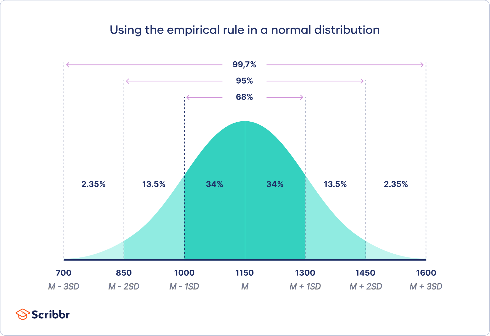
- Emparical Rule : The empirical rule, or the 68-95-99.7 rule, tells you where most of your values lie in a normal distribution:
- Around 68% of values are within 1 standard deviation from the mean.
- Around 95% of values are within 2 standard deviations from the mean.
- Around 99.7% of values are within 3 standard deviations from the mean.
-
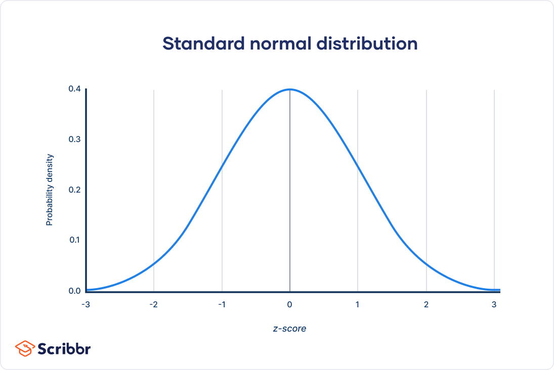
Standard Normal Distribution (Z-Distribution):
- The standard normal distribution is a specific form of the normal distribution with a mean (μ) of 0 and a standard deviation (σ) of 1.
- It's often denoted as the Z-distribution, and its values are called Z-scores.
- Z-scores indicate how many standard deviations a data point is from the mean of the distribution.
- The standard normal distribution is important in statistics because it allows us to standardize and compare data from different normal distributions.
-
Applications:
- Normal distribution assumptions are fundamental in many statistical methods and hypothesis tests.
- It's used in quality control, risk assessment, finance, and various scientific fields.
- Deviations from the normal distribution in data can indicate interesting phenomena or issues in the data collection process.
The Central Limit Theorem (CLT) is a fundamental concept in statistics that plays a crucial role in understanding the behavior of sample means or sums drawn from populations, regardless of the underlying distribution. It has widespread applications in fields ranging from social sciences to natural sciences, finance, engineering, and more. The CLT is a cornerstone in statistical theory, enabling researchers to make important inferences and draw conclusions about populations based on samples.
The Central Limit Theorem states that when independent random variables are added, their sum or average tends to follow a normal distribution, regardless of the distribution of the original variables, provided that the sample size is sufficiently large. In other words, the sampling distribution of the sample mean becomes approximately normal as the sample size increases, regardless of the shape of the population distribution.
-
Independence: The underlying random variables must be independent of each other. This condition ensures that the sample mean is not influenced by correlations between the variables.
-
Sample Size: While there is no strict threshold, a commonly accepted guideline is that the sample size should be sufficiently large (often cited as n ≥ 30). As the sample size increases, the sampling distribution of the sample mean becomes increasingly normal.
-
Cumulative Effect: The larger the sample size, the more the effects of individual deviations from the mean tend to cancel out, leading to a smoother, bell-shaped distribution.

In inferential statistics, the standard error is a critical concept that quantifies the variability or uncertainty associated with sample statistics, particularly the sample mean or sample proportion. It serves as a measure of how much the sample statistic is likely to vary from the true/actual population parameter.
The standard error of the mean (SEM) measures the average amount by which sample means would differ from the true population mean if we were to repeatedly take new samples from the same population. It takes into account both the variability of individual data points and the sample size. The formula for SEM is:
SEM = σ / √n
Where:
- σ is the population standard deviation.
- n is the sample size.
The SEM provides valuable insights into how well the sample mean estimates the true population mean. Larger sample sizes generally lead to smaller standard errors, indicating more precise estimates.
For categorical data and proportions, the standard error of the proportion estimates how much the sample proportion deviates from the true population proportion. It's particularly useful when dealing with binary outcomes (e.g., success/failure).
The formula for the standard error of the proportion is:
SE(p) = √[p * (1 - p) / n]
Where:
- p is the sample proportion.
- n is the sample size.
Like the SEM, the standard error of the proportion gives an indication of the precision of the sample proportion as an estimator of the population proportion. Larger sample sizes and proportions near 0.5 tend to result in smaller standard errors.