An opinionated Quantum Toolbox
| Quantum Tomography | Quantum Channel Analysis | Julia and JuliaGPU |
|---|---|---|
 |
 |
Warning
This is research software. Not all features are implemented or optimized.
Qutee.jl is a toolbox for studying and simulating aspects of quantum information.
This code aims to achieve the following goals:
- Construction of quantum circuits as a quantum channel
- Spectral analysis of quantum dynamical maps 1
- Riemannian optimization for quantum channel (circuit) optimization 2
- Conversion of quantum information forms (Kraus, Choi, Liouville, etc.)
- Automatic differentiation (AD)
- GPU support (with AD)
- Someday use Enzyme for AD
- And more?
For now, this package is not registered. But you can use directly from Github.
using Pkg
Pkg.add(url="https://github.com/RustyBamboo/Qutee.jl")
or
]
pkg> add https://github.com/RustyBamboo/Qutee.jl
CUDA
To use CUDA, please insure the appropriate CUDA drivers are installed. E.g., on Arch linux:
sudo pacman -S nvidia cuda
Then, add "CUDA".
using Pkg
Pkg.add("CUDA")
or
]
pkg> add CUDA
AMDGPU
To use AMDGPU, please insure the appropriate AMDGPU drivers are installed. E.g., on Arch linux:
sudo pacman -S hip-runtime-amd rocm-core
sudo pacman -S rocblas rocsparse rocsolver rocrand rocfft rocalution miopen-hip
using Pkg
Pkg.add("AMDGPU")
or
]
pkg> add AMDGPU
Use of GPUs can be found in an example notebook.
If you use Qutee.jl in your work, please consider citing
@misc{FastQuantumProcess,
  title = {Fast {{Quantum Process Tomography}} via {{Riemannian Gradient Descent}}},
  author = {Volya, Daniel and Nikitin, Andrey and Mishra, Prabhat},
  year = {2024},
  month = apr,
  number = {arXiv:2404.18840},
  eprint = {2404.18840},
  primaryclass = {quant-ph},
  publisher = {arXiv},
  doi = {10.48550/arXiv.2404.18840},
}@misc{QuantumBenchmarkingRandom,
title = {Quantum {{Benchmarking}} via {{Random Dynamical Quantum Maps}}},
author = {Volya, Daniel and Mishra, Prabhat},
year = {2024},
month = apr,
number = {arXiv:2404.18846},
eprint = {2404.18846},
primaryclass = {quant-ph},
publisher = {arXiv},
doi = {10.48550/arXiv.2404.18846},
urldate = {2024-04-30},
}In this section, we outline the functionality of the code so you can find the best tool for the job!
Generally, the code is organized into the following files:
- Optimization.jl contains the functions necessarry for performing Quantum Process Tomography via gradient descent.
- QuantumInfo.jl converts between the many representations of a quantum channel and includes methods for finding the largest eigenvalues and eigenvectors of the quantum channel.
- Qutee.jl handles the math associated with quantum channels.
- Random.jl is used for generating random channels.
A quantum channel maps one quantum state to another and is often represented as a set of matrices. The channel can be expressed in different forms to highlight different properties:
- The Kraus form is more convenient for computations. This form consists of multiple square matrices of size
$2^N\times2^N$ where$N$ is the number of qubits. The number of matrices used is known as the kraus rank. The maximum kraus rank needed to fully describe a quantum channel is$4^N$ . - The Liouville form is better for visualizing the channel.
- The Choi form can be treated as a quantum state via the Choi-jamiolkowski isomorphism. This allows us to use metrics such as state fidelity to compare two quantum channels.
Keep in mind that all of these forms include matrices consisting of complex elements. However, complex numbers can be annoying to work with, so a quantum channel can always be converted to the Pauli basis, where all elements are real.
Now let's put these ideas in practice!
using Qutee, LinearAlgebra

# First, we generate a quantum channel

N = 2  # Number of qubits

# Generate a random channel in Kraus representation
K = QuantumInfo.rand_channel(Array, 4^N, 2^N)  # Note: use CuArray as first argument if using GPU

# We could also generate a Choi matrix and then convert it to Kraus
choiChan = QuantumInfo.Random.rand_channel(Array,4^N,2^N)
krausChan = QuantumInfo.choi2kraus(choiChan)


# Now, we need a quantum state to apply our channel to

# Since the Choi representation is isomorphic to a quantum state, we can use it to generate our density state matrix!
ρ = QuantumInfo.Random.rand_channel(Array,4^div(N,2),2^(div(N,2)))
ρ = ρ/tr(ρ)  # Needs trace of 1

# Apply our channel to our quantum state
ρ = Qutee.apply(ρ,K)


# Finally, let's convert it to Liou form to visualize the channel
L = QuantumInfo.kraus2liou(K)

# Now let's demonstrate isolating a specific component of the channel, such as noise
realL = QuantumInfo.kraus2liou(QuantumInfo.rand_channel(Array,4^N,2^N))
noise = L - realL
noise = QuantumInfo.liou2pauliliou(noise)  # Displaying complex numbers is difficult, so we convert to Pauli basis

# Plot results
Understanding the long-term dynamics of a system is often important for Petz recovery maps, quantum-error correction, and measurement-induced steering for state preparation. We can ascertain how a circuit will behave in the long-term by repeatedly applying the quantum channel
QuantumInfo.jl includes two methods for finding the eigenstates of a quantum channel. For both methods, the first argument is the quantum channel and the second argument is an inital guess for the eigenvector:
power_method(A, v₀)utilizes the power method to compute the largest eigenvalue and eigenvector. While simplistic, this method can get computationally intensive and only finds the maximum eigenvalue.arnoldi2eigen(A,b,n,m)utilizes the Krylov subspace to efficiently find the largest eigenvalues and eigenvectors. As the number of iterations used increases, so does the number of eigenvalues found.
Arnoldi Analysis
The following code uses the goodness function to assess how effective certain methods are at generating eigenvectors. We will use it to test how well the arnoldi method performs.
using Qutee


function goodness(standeig, testeig, m)
    vals = zeros(ComplexF64, 1, m)  # initializes array that will hold accuracy of each eigen pair
    count = 0
    for i in 1:m  # iterates through all eigen pairs
        # compares the last (largest) eigenvalues from standeig and testeig. The closer it is to 1, the more similar the pair is.
        vals[1, i] = standeig[:, end-i+1]' * testeig[:, end-i+1]
        if norm(vals[1, i]) > 0.99  # Change this number to whatever percent similarity/accuracy you desire
            count += 1
        end
    end
    return count
end

nn = 4  # number of qubits
cases = 10 # the number of test cases
comp = zeros((2^nn)^2,1)
for j in 1:cases
	En = QuantumInfo.rand_channel(Array, 3, 2^nn)  # Random channel in Kraus representation
	Ln = QuantumInfo.kraus2liou(En)  # Convert channel to a big matrix representation
	goal = rand((2^nn)^2)  # Random start vector for arnoldi

	vals, standeig = standardeigen(Ln)  # True eigenvalues to compare to
	for i in 1:(2^nn)^2
		testvals, testeig = arnoldi2eigen(Ln,goal,(2^nn)^2,i)  # For each iteration, find arnoldi eigenvalues
		comp[i,1] += goodness(standeig,testeig,i)  # Store number of matches
	end
end
comp /= cases  # averages the results
for i in 1:(2^nn)^2  # prints result for easy copy + paste to store for later
	print(comp[i,1])
	print(", ")
end

# Plotting the results
By plotting the results, we can see that for any number of qubits, the first eigenvalue tends to be found fairly quickly (m < 10). However, finding any more than that takes significantly longer. Also, it is interesting how sporadic the number of eigenvalues found is.
CUDA
A small benchmark that compares CPU and CUDA in
- Matrix-matrix multiplication
- Finding the largest eigenpair via the power method
using LinearAlgebra, Pkg, Plots, BenchmarkTools, CUDA
using Qutee

function random_vector(K)
	n,m,_ = size(K)
	v = rand(n,m) + im * rand(n,m)
    v /= norm(v)
end

K_list = [QuantumInfo.rand_channel(CuArray,2,2^i) for i in 1:11]
v_list = [random_vector(K) for K in K_list]

cpu_times = [@elapsed K_list[i] * v_list[i] for i in 1:length(K_list)]
gpu_times = [CUDA.@elapsed cu(K_list[i]) * cu(v_list[i]) for i in 1:length(K_list)]
p1 = plot([cpu_times, gpu_times], labels=["CPU" "CUDA"], title="Matrix-Matrix Multiplication", xlabel="# of Qubits", ylabel="Time [s]", markershape=:xcross)
savefig(p1, "benchmark1.png")

cpu_times_power = [@elapsed QuantumInfo.power_method(K_list[i], v_list[i], 50) for i in 1:length(K_list)]
gpu_times_power = [@elapsed QuantumInfo.power_method(cu(K_list[i]), cu(v_list[i]), 50) for i in 1:length(K_list)]
p2 = plot([cpu_times_power, gpu_times_power], labels=["CPU" "CUDA"], title="Power Method (50 Iterations)", xlabel="# of Qubits", ylabel="Time [s]", markershape=:xcross)
savefig(p2, "benchmark2.png")

Given an initial and final quantum state, the goal of Quantum Process Tomography(QPT) is to figure out what the quantum channel is. While methods such as linear inversion and convex hull optimization are used in other QPT libraries, they are too slow for systems larger than 3 qubits and require the informationally-complete set of measurements in order to produce a solution, which can get costly. Instead, Optimization.jl utilizes gradient descent to find the quantum channel.
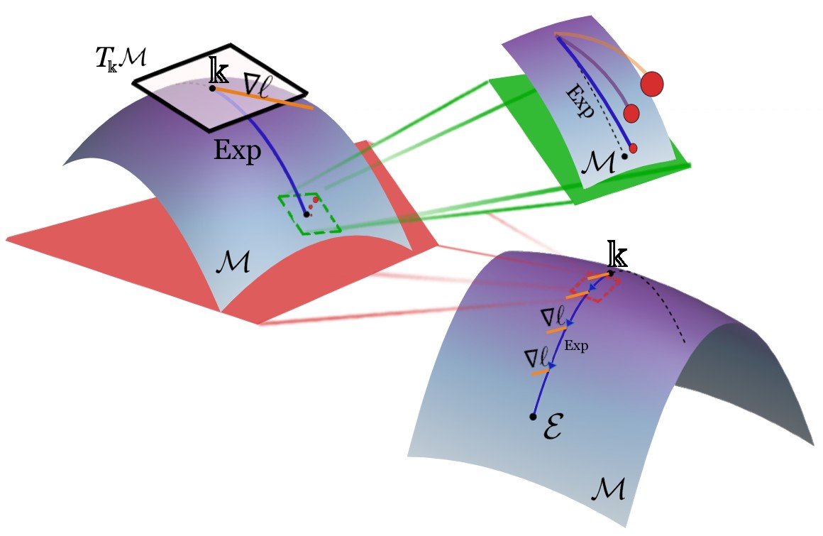
However, simple gradient descent will not suffice! That is because gradient descent assumes a Euclidean geometry, but quantum channels exist in the Steifel manifold. Thus, the optimizer's steps must be projected back onto the Stiefel manifold, which is approximated through a retraction.
Qutee offers a few methods for QPT:
optimize(K, f)uses naive gradient descent. You can specify the retraction use as eitherretractionorqr_retractionoptimize_adam(K, f)uses Adam-Cayley gradient descent, which implicitly performs the retraction as it steps.AdamCayley(K)is a wrapper class foroptimize_adam(K,f)that allows for easier implementation!
Circuit Optimization
using Qutee

# 2-qubit operation: Qubit reset and Identity
op = (QuantumInfo.R ⊗ [1 0; 0 1])

# A vector of random 2-qubit gates (4x4 unitary matrices)
rand_U = [reshape(QuantumInfo.rand_channel(Array,1,2^2), (2^2,2^2)) for _ in 1:3]

# Construction of the circuit
function circuit(U)
	C = mapreduce(x->op⊙x, ⊙, U)
	return C
end

# The loss function that we wish to optimize. You can compare to whatever matrix you want.
# For reference, here I use a simple example where we compare to the identity matrix.
function circuit_error(U)
    C = circuit(U)  # Creates a circuit from our matrix
	C_L = QuantumInfo.kraus2liou(C)  # Converts the circuit to a form we can work with
	return norm(C_L - I)  # Example loss function
end

# Optimize using gradient descent over the Stiefel Manifold
out_u, history_u = QuantumInfo.Optimization.optimize(rand_U, circuit_error, 500; η=0.2, decay_factor=0.9, decay_step=10)

- Daniel Volya
- Andrey Nikitin
Footnotes
-
D. Volya and P. Mishra, “Quantum Benchmarking via Random Dynamical Quantum Maps” arXiv, Apr. 29, 2024. doi: 10.48550/arXiv.2404.18846. ↩
-
D. Volya, A. Nikitin, and P. Mishra, “Fast Quantum Process Tomography via Riemannian Gradient Descent.” arXiv, Apr. 29, 2024. doi: 10.48550/arXiv.2404.18840. ↩