![]()
Drive folder that contains the dataset, the model and the colab notebook
- Summary
- Siamese Neural Networks to Compare two Signatures
- Data Generation Approach
- Training the model
- Verification of the model
This is the Model for the project Handwritten Digital, for SWAT - Platzi Master. Handwritten Digital was divided in three projects, these three projects were build by an amazing team, that is described next.

Signature verification and forgery detection is the process of verifying signatures automatically and instantly to determine whether the signature is real or not. There are two main kinds of signature verification: static and dynamic. Static, or off-line verification is the process of verifying a document signature after it has been made, while dynamic or on-line verificationtakes place as a person creates his/her signature on a digital tablet or a similar device.
In this project, the process will be entirely off-line, therefore, the user will have to upload the photo of his/her signature in order to check how similar are the signatures in the database versus the photo recently uploaded. If the comparison is over 90% the signature is considered reliable and proceed to certified the document.
# the CNN is the diagram
feature_vector = tf.keras.Sequential()
feature_vector.add(tf.keras.layers.Conv2D(2,3, activation='relu', input_shape=(150,150,3)))
feature_vector.add(tf.keras.layers.BatchNormalization())
feature_vector.add(tf.keras.layers.MaxPool2D((2,2)))
feature_vector.add(tf.keras.layers.Flatten())
feature_vector.add(tf.keras.layers.Dropout(0.2))
feature_vector.add(tf.keras.layers.Dense(2, activation='relu'))-
Keras Conv2D is a 2D Convolution Layer, this layer creates a convolution kernel that is wind with layers input which helps produce a tensor of outputs.
- The kernel is an integer or tuple/list of 2 integers, specifying the height and width of the 2D convolution window. In this case the size of the Kernel is 2.
- The stride is an integer or tuple/list of 2 integers, specifying the “step” of the convolution along with the height and width of the input volume. Its default value is always set to (1, 1) which means that the given Conv2D filter is applied to the current location of the input volume and the given filter takes a 1-pixel step to the right and again the filter is applied to the input volume and it is performed until we reach the far right border of the volume in which we are moving our filter. In this case the size of the stride is 3.
- The activation function is simply a convenience parameter which allows you to supply a string, which specifies the name of the activation function you want to apply after performing the convolution. In this case is the relu function.
- Input shape, this argument is at the first layer in a model, in this case it means that the input for the CNN it's going to be 150x150 pixels with the channels RGB, that's why the number 3 is in there.
-
BatchNormalization: Normalize the activations of the previous layer at each batch, i.e. applies a transformation that maintains the mean activation close to 0 and the activation standard deviation close to 1. Importantly, batch normalization works differently during training and during inference.
- During training (i.e. when using fit() or when calling the layer/model with the argument training=True), the layer normalizes its output using the mean and standard deviation of the current batch of inputs. That is to say, for each channel being normalized, the layer returns
(batch - mean(batch)) / (var(batch) + epsilon) * gamma + beta, where:- epsilon is small constant (configurable as part of the constructor arguments)
- gamma is a learned scaling factor (initialized as 1), which can be disabled by passing scale=False to the constructor.
- beta is a learned offset factor (initialized as 0), which can be disabled by passing center=False to the constructor.
- During inference (i.e. when using evaluate() or predict() or when calling the layer/model with the argument training=False (which is the default), the layer normalizes its output using a moving average of the mean and standard deviation of the batches it has seen during training. That is to say, it returns
(batch - self.moving_mean) / (self.moving_var + epsilon) * gamma + beta.- self.moving_mean and self.moving_var are non-trainable variables that are updated each time the layer in called in training mode, as such:
moving_mean = moving_mean * momentum + mean(batch) * (1 - momentum)moving_var = moving_var * momentum + var(batch) * (1 - momentum)
- self.moving_mean and self.moving_var are non-trainable variables that are updated each time the layer in called in training mode, as such:
As such, the layer will only normalize its inputs during inference after having been trained on data that has similar statistics as the inference data.
- During training (i.e. when using fit() or when calling the layer/model with the argument training=True), the layer normalizes its output using the mean and standard deviation of the current batch of inputs. That is to say, for each channel being normalized, the layer returns
-
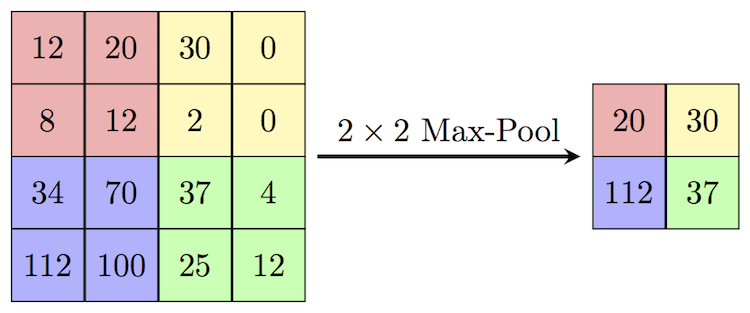
MaxPool2d: We use Max Pooling to reduce the spatial dimensions of the output volume.
-
Flatten: Flattens the input. Does not affect the batch size. It works converting a matrix into an array.
-
Dropout: The Dropout layer randomly sets input units to 0 with a frequency of rate at each step during training time, which helps prevent overfitting. Inputs not set to 0 are scaled up by 1/(1 - rate) such that the sum over all inputs is unchanged. The rate is a float between 0 and 1 (in this case is 0.2), this is the fraction of the input units to drop.
-
Dense: Dense layer is the regular deeply connected neural network layer. It is most common and frequently used layer. In this case we use two arguments, units and the activation function.
- units: Positive integer, dimensionality of the output space.
- activation: Activation function to use. If you don't specify anything, no activation is applied (ie. "linear" activation: a(x) = x).
Now, this is the summary for the CNN created.
Model: "sequential"
_________________________________________________________________
Layer (type)                 Output Shape              Param #
=================================================================
conv2d (Conv2D)              (None, 148, 148, 2)       56
_________________________________________________________________
batch_normalization (BatchNo (None, 148, 148, 2)       8
_________________________________________________________________
max_pooling2d (MaxPooling2D) (None, 74, 74, 2)         0
_________________________________________________________________
flatten (Flatten)            (None, 10952)             0
_________________________________________________________________
dropout (Dropout)            (None, 10952)             0
_________________________________________________________________
dense (Dense)                (None, 2)                 21906
=================================================================
Total params: 21,970
Trainable params: 21,966
Non-trainable params: 4
# creating the siamese network
im_a = tf.keras.layers.Input(shape=(150,150,3))
im_b = tf.keras.layers.Input(shape=(150,150,3))

encoded_a = feature_vector(im_a)
encoded_b = feature_vector(im_b)

combined = tf.keras.layers.concatenate([encoded_a, encoded_b])
combined = tf.keras.layers.BatchNormalization()(combined)
combined = tf.keras.layers.Dense(8, activation = 'linear')(combined)
combined = tf.keras.layers.BatchNormalization()(combined)
combined = tf.keras.layers.Activation('relu')(combined)
combined = tf.keras.layers.Dense(1, activation = 'sigmoid')(combined)

sm = tf.keras.Model(inputs=[im_a, im_b], outputs=[combined])
The very first thing to do is set the shape of the inputs, here are considered as im_a (image a) and im_b (image b).
Then, these two features are encoded with the CNN previously described.
Now, the output is configured, in a variable named combined, this is the Siamese Neural Network. Combined use the next layers:
- Concatenate: Layer that concatenates a list of inputs. It takes as input a list of tensors, all of the same shape except for the concatenation axis, and returns a single tensor that is the concatenation of all inputs.
- BatchNormalization: Previously described.
- Dense: Previously described.
- Activation: Applies an activation function to an output. In this case the activation function is relu.
Now we create the siamese Neural Nework with Model. Model groups layers into an object with training and inference features. In this case, the inputs are the CNN for the two images uploaded, and the output is the combined variable.
sm = tf.keras.Model(inputs=[im_a, im_b], outputs=[combined])
Now, this is the summary for the model.
Layer (type)                    Output Shape         Param #     Connected to
==================================================================================================
input_1 (InputLayer)            [(None, 150, 150, 3) 0
__________________________________________________________________________________________________
input_2 (InputLayer)            [(None, 150, 150, 3) 0
__________________________________________________________________________________________________
sequential (Sequential)         (None, 2)            21970       input_1[0][0]
                                                                 input_2[0][0]
__________________________________________________________________________________________________
concatenate (Concatenate)       (None, 4)            0           sequential[0][0]
                                                                 sequential[1][0]
__________________________________________________________________________________________________
batch_normalization_1 (BatchNor (None, 4)            16          concatenate[0][0]
__________________________________________________________________________________________________
dense_1 (Dense)                 (None, 8)            40          batch_normalization_1[0][0]
__________________________________________________________________________________________________
batch_normalization_2 (BatchNor (None, 8)            32          dense_1[0][0]
__________________________________________________________________________________________________
activation (Activation)         (None, 8)            0           batch_normalization_2[0][0]
__________________________________________________________________________________________________
dense_2 (Dense)                 (None, 1)            9           activation[0][0]
==================================================================================================
Total params: 22,067
Trainable params: 22,039
Non-trainable params: 28
sm.compile(optimizer='adam', loss = 'binary_crossentropy', metrics = ['accuracy'])
Compile configures the model for training. Compile receives the next arguments:
- optimizer: String (name of optimizer) or optimizer instance. See tf.keras.optimizers.
- loss: String (name of objective function), objective function or tf.keras.losses.Loss instance. It returns a weighted loss float tensor.
- metrics: List of metrics to be evaluated by the model during training and testing. Each of this can be a string (name of a built-in function)
In this approach, we try to setup a dataset where we cross multiply each signature with other number signature. The inputs and the outputs must be the same size.
Now, the function generate_dataset_approach_two, returns eight variables, x_train, y_train, x_test, y_test, x_val, y_val, pairs, ls.
The most importants here are the six first variables, with them we can train the model.
history = sm.fit([x_train[:,0], x_train[:,1]], y_train, epochs=10, validation_data=([x_test[:,0], x_test[:,1]], y_test))To train a model it is used the fit function in keras. it receives 4 parameters:
- First the training set, it is configured in the list
[x_train[:,0], x_train[:,1]]. - Then the training variable in
y_train. - The epochs, this is the number of iterations the NN (Neural Network) is going to be trained. For this case we use 10 epochs.
- Finally, the validation data, it receives the test for the inputs (original and forged), it is configured in the list
[x_test[:,0], x_test[:,1]], and the results in the variabley_test.
The result of the training is described next.
Epoch 1/10
89/89 [==============================] - 56s 625ms/step - loss: 0.3727 - accuracy: 0.9111 - val_loss: 0.2923 - val_accuracy: 0.9291
Epoch 2/10
89/89 [==============================] - 55s 622ms/step - loss: 0.2304 - accuracy: 0.9207 - val_loss: 0.1473 - val_accuracy: 0.9291
Epoch 3/10
89/89 [==============================] - 56s 628ms/step - loss: 0.1524 - accuracy: 0.9221 - val_loss: 0.1400 - val_accuracy: 0.9299
Epoch 4/10
89/89 [==============================] - 55s 623ms/step - loss: 0.1072 - accuracy: 0.9720 - val_loss: 0.1177 - val_accuracy: 0.9992
Epoch 5/10
89/89 [==============================] - 56s 628ms/step - loss: 0.0774 - accuracy: 1.0000 - val_loss: 0.0443 - val_accuracy: 0.9936
Epoch 6/10
89/89 [==============================] - 56s 627ms/step - loss: 0.0524 - accuracy: 1.0000 - val_loss: 0.0307 - val_accuracy: 0.9992
Epoch 7/10
89/89 [==============================] - 56s 629ms/step - loss: 0.0334 - accuracy: 1.0000 - val_loss: 0.0207 - val_accuracy: 0.9992
Epoch 8/10
89/89 [==============================] - 56s 626ms/step - loss: 0.0235 - accuracy: 1.0000 - val_loss: 0.0151 - val_accuracy: 0.9992
Epoch 9/10
89/89 [==============================] - 56s 631ms/step - loss: 0.0197 - accuracy: 1.0000 - val_loss: 0.0155 - val_accuracy: 0.9992
Epoch 10/10
89/89 [==============================] - 57s 636ms/step - loss: 0.0148 - accuracy: 1.0000 - val_loss: 0.0100 - val_accuracy: 0.9992
According to the result of the model, especially the loss function, both for training and validation it is important to know the behaviour of these two, that is why is important plotting, it shows in an easy way how is the model acting with the data that is entered.

As we can see, the loss for the validation data is beneath the loss for the training data, this result is very interesting, for we can say that the algorithm is actually learning and analyzing patterns in the signatures.
The very first thing to do is saving the model into the hard drive with the function save in keras.
# save model and architecture to single file
sm.save("prediction-model.h5")# load and evaluate a saved model
import tensorflow as tf
from tensorflow.keras.preprocessing.image import load_img, img_to_array
from tensorflow.keras.models import load_model
import matplotlib.pyplot as plt
%matplotlib inlinefirst, the libraries to load the program must be imported.
# load model
model = load_model('prediction-model.h5',compile=True)
Now that the model is loaded and lives in memory, we can begin to use it, but first, we need to know the summary for it.
Layer (type)                    Output Shape         Param #     Connected to
==================================================================================================
input_1 (InputLayer)            [(None, 150, 150, 3) 0
__________________________________________________________________________________________________
input_2 (InputLayer)            [(None, 150, 150, 3) 0
__________________________________________________________________________________________________
sequential (Sequential)         (None, 2)            21970       input_1[0][0]
                                                                 input_2[0][0]
__________________________________________________________________________________________________
concatenate (Concatenate)       (None, 4)            0           sequential[0][0]
                                                                 sequential[1][0]
__________________________________________________________________________________________________
batch_normalization_1 (BatchNor (None, 4)            16          concatenate[0][0]
__________________________________________________________________________________________________
dense_1 (Dense)                 (None, 8)            40          batch_normalization_1[0][0]
__________________________________________________________________________________________________
batch_normalization_2 (BatchNor (None, 8)            32          dense_1[0][0]
__________________________________________________________________________________________________
activation (Activation)         (None, 8)            0           batch_normalization_2[0][0]
__________________________________________________________________________________________________
dense_2 (Dense)                 (None, 1)            9           activation[0][0]
==================================================================================================
Total params: 22,067
Trainable params: 22,039
Non-trainable params: 28
Now that we know the parameters and the trainable parameters for the Siamese Neural Network, we upload the test data and print it to know what's the genuine, real and the forged.
# Test data
test_path = './Input/my_test/'
genuine = test_path +'test-original.jpg'
real = test_path + 'test-real.jpg'
forged = test_path + 'test-forge.jpg'

# Ploting the data
fig, axs = plt.subplots(3, 1, constrained_layout=True)

# Genuine
gen_img = load_img(genuine,color_mode='rgb', target_size=(150,150))
axs[0].imshow(gen_img)
axs[0].set_title('Genuine')
gen_img = img_to_array(gen_img)
gen_img = tf.expand_dims(gen_img,0)

# Real
r_img = load_img(real,color_mode='rgb', target_size=(150,150))
axs[1].imshow(r_img)
axs[1].set_title('real')
r_img = img_to_array(r_img)
r_img = tf.expand_dims(r_img,0)

# Falsa
for_img = load_img(forged,color_mode='rgb', target_size=(150,150))
axs[2].imshow(for_img)
axs[2].set_title('Forged')
for_img = img_to_array(for_img)
for_img = tf.expand_dims(for_img,0)
plt.show()
Now that we know wich image is the genuine, real and forged, it's time to test the model, for that the model has a single function very easy to use, predict, it receives two params:
- The first is the genuine, or the one which is the base of the comparison.
- The other is the data that's going to be compared.
The result is a number between 0 to 1, in order to use properly this model, we use the 0.9 as the base to say that the signature is real, below 0.9 we say that the signature is a forge.
real_deepsign_model = model.predict([gen_img,r_img])
print(f'Predicción real: {real_deepsign_model}')

forged_deepsign_model = model.predict([gen_img,for_img])
print(f'Predicción falsificación: {forged_deepsign_model}')

> Predicción real: [[0.9257821]]
> Predicción falsificación: [[0.898185]]
According to the results, we can say that it is correct, due to the real is above 0.9, and the forged is below 0.9.