This repository has been archived by the owner on Jul 19, 2023. It is now read-only.
New MOLFiniteDifference Discretization #349
Merged
Conversation
This file contains bidirectional Unicode text that may be interpreted or compiled differently than what appears below. To review, open the file in an editor that reveals hidden Unicode characters.
Learn more about bidirectional Unicode characters
Member
 ChrisRackauckas
commented
ChrisRackauckas
commented
Mar 27, 2021
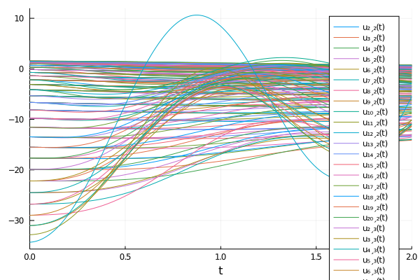
```julia
using ModelingToolkit, DiffEqOperators, LinearAlgebra

# 3D PDE
@parameters t x y
@variables u(..)
Dxx = Differential(x)^2
Dyy = Differential(y)^2
Dt = Differential(t)
t_min= 0.
t_max = 2.0
x_min = 0.
x_max = 2.
y_min = 0.
y_max = 2.

# 3D PDE
eq  = Dt(u(t,x,y)) ~ Dxx(u(t,x,y)) + Dyy(u(t,x,y))

analytic_sol_func(t,x,y) = exp(x+y)*cos(x+y+4t)
# Initial and boundary conditions
bcs = [u(t_min,x,y) ~ analytic_sol_func(t_min,x,y),
       u(t,x_min,y) ~ analytic_sol_func(t,x_min,y),
       u(t,x_max,y) ~ analytic_sol_func(t,x_max,y),
       u(t,x,y_min) ~ analytic_sol_func(t,x,y_min),
       u(t,x,y_max) ~ analytic_sol_func(t,x,y_max)]

# Space and time domains
domains = [t ∈ IntervalDomain(t_min,t_max),
           x ∈ IntervalDomain(x_min,x_max),
           y ∈ IntervalDomain(y_min,y_max)]
pdesys = PDESystem([eq],bcs,domains,[t,x,y],[u(t,x,y)])

# Method of lines discretization
dx = 0.1; dy = 0.2
discretization = MOLFiniteDifference([x=>dx,y=>dy],t)
prob = ModelingToolkit.discretize(pdesys,discretization)

using OrdinaryDiffEq
sol = solve(prob,Tsit5())
using Plots
plot(sol)
savefig("plot.png")
```
|
|
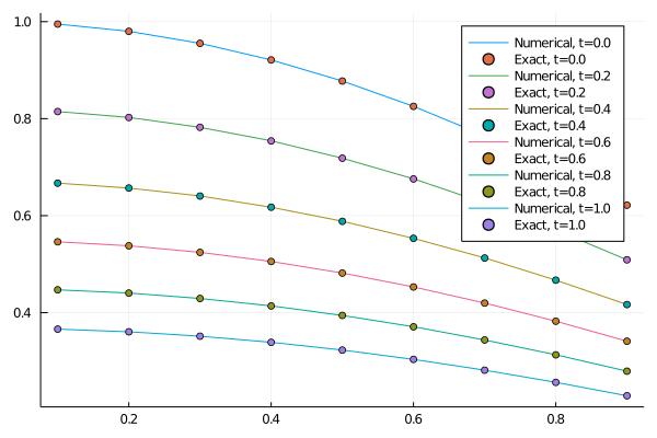
using OrdinaryDiffEq, ModelingToolkit, DiffEqOperators
# Method of Manufactured Solutions: exact solution
u_exact = (x,t) -> exp.(-t) * cos.(x)

# Parameters, variables, and derivatives
@parameters t x
@variables u(..)
Dt = Differential(t)
Dxx = Differential(x)^2

# 1D PDE and boundary conditions
eq  = Dt(u(t,x)) ~ Dxx(u(t,x))
bcs = [u(0,x) ~ cos(x),
        u(t,0) ~ exp(-t),
        u(t,1) ~ exp(-t) * cos(1)]

# Space and time domains
domains = [t ∈ IntervalDomain(0.0,1.0),
           x ∈ IntervalDomain(0.0,1.0)]

# PDE system
pdesys = PDESystem(eq,bcs,domains,[t,x],[u(t,x)])

# Method of lines discretization
dx = 0.1
order = 2
discretization = MOLFiniteDifference([x=>dx],t)

# Convert the PDE problem into an ODE problem
prob = discretize(pdesys,discretization)

# Solve ODE problem
using OrdinaryDiffEq
sol = solve(prob,Tsit5(),saveat=0.2)

# Plot results and compare with exact solution
x = (0:dx:1)[2:end-1]
t = sol.t

using Plots
plt = plot()

for i in 1:length(t)
    plot!(x,sol.u[i],label="Numerical, t=$(t[i])")
    scatter!(x, u_exact(x, t[i]),label="Exact, t=$(t[i])")
end
display(plt)
savefig("plot.png")
|
|
Neumann: using OrdinaryDiffEq, ModelingToolkit, DiffEqOperators
# Method of Manufactured Solutions: exact solution
u_exact = (x,t) -> exp.(-t) * cos.(x)
# Parameters, variables, and derivatives
@parameters t x
@variables u(..)
Dt = Differential(t)
Dx = Differential(x)
Dxx = Differential(x)^2
# 1D PDE and boundary conditions
eq = Dt(u(t,x)) ~ Dxx(u(t,x))
bcs = [u(0,x) ~ cos(x),
Dx(u(t,0)) ~ 0.0,
Dx(u(t,1)) ~ -exp(-t) * sin(1)]
# Space and time domains
domains = [t ∈ IntervalDomain(0.0,1.0),
x ∈ IntervalDomain(0.0,1.0)]
# PDE system
pdesys = PDESystem(eq,bcs,domains,[t,x],[u(t,x)])
# Method of lines discretization
# Need a small dx here for accuracy
dx = 0.01
order = 2
discretization = MOLFiniteDifference([x=>dx],t)
# Convert the PDE problem into an ODE problem
prob = discretize(pdesys,discretization)
# Solve ODE problem
using OrdinaryDiffEq
sol = solve(prob,Tsit5(),saveat=0.2)
# Plot results and compare with exact solution
x = (0:dx:1)[2:end-1]
t = sol.t
using Plots
plt = plot()
for i in 1:length(t)
plot!(x,sol.u[i],label="Numerical, t=$(t[i])",lw=12)
scatter!(x, u_exact(x, t[i]),label="Exact, t=$(t[i])")
end
display(plt)
savefig("plot.png")
|
|
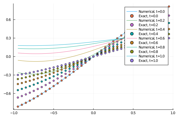
Given the implementation, Robin comes for free, but curiously: using OrdinaryDiffEq, ModelingToolkit, DiffEqOperators
# Method of Manufactured Solutions
u_exact = (x,t) -> exp.(-t) * sin.(x)
# Parameters, variables, and derivatives
@parameters t x
@variables u(..)
Dt = Differential(t)
Dx = Differential(x)
Dxx = Differential(x)^2
# 1D PDE and boundary conditions
eq = Dt(u(t,x)) ~ Dxx(u(t,x))
bcs = [u(0,x) ~ sin(x),
u(t,-1.0) + 3Dx(u(t,-1.0)) ~ exp(-t) * (sin(-1.0) + 3cos(-1.0)),
u(t,1.0) + Dx(u(t,1.0)) ~ exp(-t) * (sin(1.0) + cos(1.0))]
# Space and time domains
domains = [t ∈ IntervalDomain(0.0,1.0),
x ∈ IntervalDomain(-1.0,1.0)]
# PDE system
pdesys = PDESystem(eq,bcs,domains,[t,x],[u(t,x)])
# Method of lines discretization
# Need a small dx here for accuracy
dx = 0.05
order = 2
discretization = MOLFiniteDifference([x=>dx],t)
# Convert the PDE problem into an ODE problem
prob = discretize(pdesys,discretization)
# Solve ODE problem
using OrdinaryDiffEq
sol = solve(prob,Tsit5(),saveat=0.2)
# Plot results and compare with exact solution
x = (-1:dx:1)[2:end-1]
t = sol.t
using Plots
plt = plot()
for i in 1:length(t)
plot!(x,sol.u[i],label="Numerical, t=$(t[i])")
scatter!(x, u_exact(x, t[i]),label="Exact, t=$(t[i])")
end
display(plt)
savefig("plot.png")
@tinosulzer how sure are you on that Robin BC analytical solution? I would think there's a sign error in there, since the direction of discretization is the same code from the Neumann which works, so I'm not sure what would go wrong if Dirichlet and Neumann work in this implementation. |
|
|
Requires JuliaSymbolics/SymbolicUtils.jl#251 |
This was referenced Mar 28, 2021
Sign up for free
to subscribe to this conversation on GitHub.
Already have an account?
Sign in.
Add this suggestion to a batch that can be applied as a single commit.
This suggestion is invalid because no changes were made to the code.
Suggestions cannot be applied while the pull request is closed.
Suggestions cannot be applied while viewing a subset of changes.
Only one suggestion per line can be applied in a batch.
Add this suggestion to a batch that can be applied as a single commit.
Applying suggestions on deleted lines is not supported.
You must change the existing code in this line in order to create a valid suggestion.
Outdated suggestions cannot be applied.
This suggestion has been applied or marked resolved.
Suggestions cannot be applied from pending reviews.
Suggestions cannot be applied on multi-line comments.
Suggestions cannot be applied while the pull request is queued to merge.
Suggestion cannot be applied right now. Please check back later.