
Wasserstein Distance is a measure of the distance between two probability distributions. It is also called Earth Mover’s distance, short for EM distance, because informally it can be interpreted as the minimum energy cost of moving and transforming a pile of dirt in the shape of one probability distribution to the shape of the other distribution. The cost is quantified by: the amount of dirt moved x the moving distance.
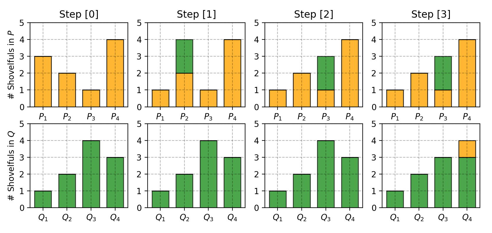
Let us first look at a simple case where the probability domain is discrete. For example, suppose we have two distributions P and Q, each has four piles of dirt and both have ten shovelfuls of dirt in total. The numbers of shovelfuls in each dirt pile are assigned as follows:
P1=3,P2=2,P3=1,P4=4Q1=1,Q2=2,Q3=4,Q4=3
In order to change P to look like Q, as illustrated in Fig. 7, we:
- First move 2 shovelfuls from P1 to P2 => (P1,Q1) match up.
- Then move 2 shovelfuls from P2 to P3 => (P2,Q2) match up.
- Finally move 1 shovelfuls from Q3 to Q4 => (P3,Q3) and (P4,Q4) match up.
If we label the cost to pay to make Pi and Qi match as δi, we would have δi+1=δi+Pi−Qi and in the example:
δ0δ1δ2δ3δ4=0=0+3−1=2=2+2−2=2=2+1−4=−1=−1+4−3=0
Finally the Earth Mover’s distance is W=∑|δi|=5.
When dealing with the continuous probability domain, the distance formula becomes:
W(pr,pg)=infγ∼Π(pr,pg)E(x,y)∼γ[∥x−y∥] In the formula above, Π(pr,pg) is the set of all possible joint probability distributions between pr and pg. One joint distribution γ∈Π(pr,pg) describes one dirt transport plan, same as the discrete example above, but in the continuous probability space. Precisely γ(x,y) states the percentage of dirt should be transported from point x to y so as to make x follows the same probability distribution of y. That’s why the marginal distribution over x adds up to pg, ∑xγ(x,y)=pg(y) (Once we finish moving the planned amount of dirt from every possible x to the target y, we end up with exactly what y has according to pg.) and vice versa ∑yγ(x,y)=pr(x).
When treating x as the starting point and y as the destination, the total amount of dirt moved is γ(x,y) and the travelling distance is ∥x−y∥ and thus the cost is γ(x,y)⋅∥x−y∥. The expected cost averaged across all the (x,y) pairs can be easily computed as:
∑x,yγ(x,y)∥x−y∥=Ex,y∼γ∥x−y∥
Finally, we take the minimum one among the costs of all dirt moving solutions as the EM distance. In the definition of Wasserstein distance, the inf (infimum, also known as greatest lower bound) indicates that we are only interested in the smallest cost.
It is intractable to exhaust all the possible joint distributions in Π(pr,pg) to compute infγ∼Π(pr,pg). Thus the authors proposed a smart transformation of the formula based on the Kantorovich-Rubinstein duality to:
W(pr,pg)=1Ksup∥f∥L≤KEx∼pr[f(x)]−Ex∼pg[f(x)]
where sup (supremum) is the opposite of inf (infimum); we want to measure the least upper bound or, in even simpler words, the maximum value.
The function f in the new form of Wasserstein metric is demanded to satisfy ∥f∥L≤K, meaning it should be K-Lipschitz continuous.
A real-valued function f:R→R is called K-Lipschitz continuous if there exists a real constant K≥0 such that, for all x1,x2∈R,
|f(x1)−f(x2)|≤K|x1−x2|
Here K is known as a Lipschitz constant for function f(.). Functions that are everywhere continuously differentiable is Lipschitz continuous, because the derivative, estimated as |f(x1)−f(x2)||x1−x2|, has bounds. However, a Lipschitz continuous function may not be everywhere differentiable, such as f(x)=|x|.
Explaining how the transformation happens on the Wasserstein distance formula is worthy of a long post by itself, so I skip the details here. If you are interested in how to compute Wasserstein metric using linear programming, or how to transfer Wasserstein metric into its dual form according to the Kantorovich-Rubinstein Duality, read this awesome post.
Suppose this function f comes from a family of K-Lipschitz continuous functions, {fw}w∈W, parameterized by w. In the modified Wasserstein-GAN, the “discriminator” model is used to learn w to find a good fw and the loss function is configured as measuring the Wasserstein distance between pr and pg.
L(pr,pg)=W(pr,pg)=maxw∈WEx∼pr[fw(x)]−Ez∼pr(z)[fw(gθ(z))]
Thus the “discriminator” is not a direct critic of telling the fake samples apart from the real ones anymore. Instead, it is trained to learn a K-Lipschitz continuous function to help compute Wasserstein distance. As the loss function decreases in the training, the Wasserstein distance gets smaller and the generator model’s output grows closer to the real data distribution.
One big problem is to maintain the K-Lipschitz continuity of fw during the training in order to make everything work out. The paper presents a simple but very practical trick: After every gradient update, clamp the weights w to a small window, such as [−0.01,0.01], resulting in a compact parameter space W and thus fw obtains its lower and upper bounds to preserve the Lipschitz continuity.
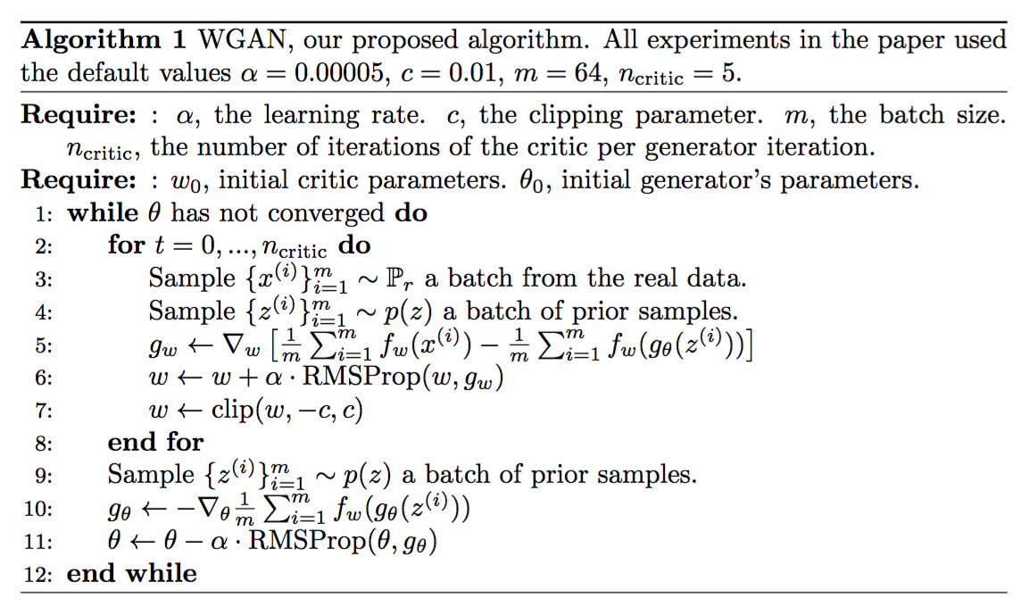
Fig. 9. Algorithm of Wasserstein generative adversarial network. (Image source: Arjovsky, Chintala, & Bottou, 2017.)
Compared to the original GAN algorithm, the WGAN undertakes the following changes:
After every gradient update on the critic function, clamp the weights to a small fixed range, [−c,c]. Use a new loss function derived from the Wasserstein distance, no logarithm anymore. The “discriminator” model does not play as a direct critic but a helper for estimating the Wasserstein metric between real and generated data distribution. Empirically the authors recommended RMSProp optimizer on the critic, rather than a momentum based optimizer such as Adam which could cause instability in the model training. I haven’t seen clear theoretical explanation on this point through. Sadly, Wasserstein GAN is not perfect. Even the authors of the original WGAN paper mentioned that “Weight clipping is a clearly terrible way to enforce a Lipschitz constraint” (Oops!). WGAN still suffers from unstable training, slow convergence after weight clipping (when clipping window is too large), and vanishing gradients (when clipping window is too small).
Some improvement, precisely replacing weight clipping with gradient penalty, has been discussed in Gulrajani et al. 2017. Our implementation is done in the keras framework. It uses the MNIST database
