王世兴
2013301020050
Problem 5.7
Write two programs to solve the capacitor problem of Figure 5.6 and 5.7, one using Jacobi method and one using simultaneous over relaxation (SOR) algrithem . For a fixed accuracy compare the number of iterations,
The partial differential equation is of physicists' great interest for its widely applicaiton in decribing physical systems. Jacobi method and simultaneous over relaxation (SOR) method are two algrithm that keep a balance of the simplicity for comprehension and accuracy of computation. Thanks to Li Yao's code, we realized the two algorithm with Python in calculating a finite parallel capacitor system.
In numerical linear algebra, the Jacobi method (or Jacobi iterative method) is an algorithm for determining the solutions of a diagonally dominant system of linear equations. Each diagonal element is solved for, and an approximate value is plugged in. The process is then iterated until it converges. This algorithm is a stripped-down version of the Jacobi transformation method of matrix diagonalization. The method is named after Carl Gustav Jacob Jacobi.
In numerical linear algebra, the method of successive over-relaxation (SOR) is a variant of the Gauss–Seidel method for solving a linear system of equations, resulting in faster convergence. A similar method can be used for any slowly converging iterative process.
It was devised simultaneously by David M. Young, Jr. and by H. Frankel in 1950 for the purpose of automatically solving linear systems on digital computers. Over-relaxation methods had been used before the work of Young and Frankel. An example is the method of Lewis Fry Richardson, and the methods developed by R. V. Southwell. However, these methods were designed for computation by human calculators, and they required some expertise to ensure convergence to the solution which made them inapplicable for programming on digital computers. These aspects are discussed in the thesis of David M. Young, Jr.
-
Initial condition
At first we give a guess about the system with all the points zero other than the boundary conditions. Thus we need a quick way to creat a two-dimension zero list. Fistly we used the list calculation[[0.0]*m]*n
However, this method proved inappropriate because when we want to change the value of some elements in one row, the elements at the same position in other rows will also be changed. The reason is not clear at present. So we use the following code
[[0.0 for i in range(m)] for j in range(n)]
-
Interating Number and Judge for Convergence
To measure the complexity of the paorgram we need to define the how we can claim that the algorithm is at convergence, then we defined the interating numberself.Nto see how many cycle we need to reach the convergence. We define the sum of the difference at each point before and after one turn asself.delta.self.Nis added one to itself every time the program enters the cycle.
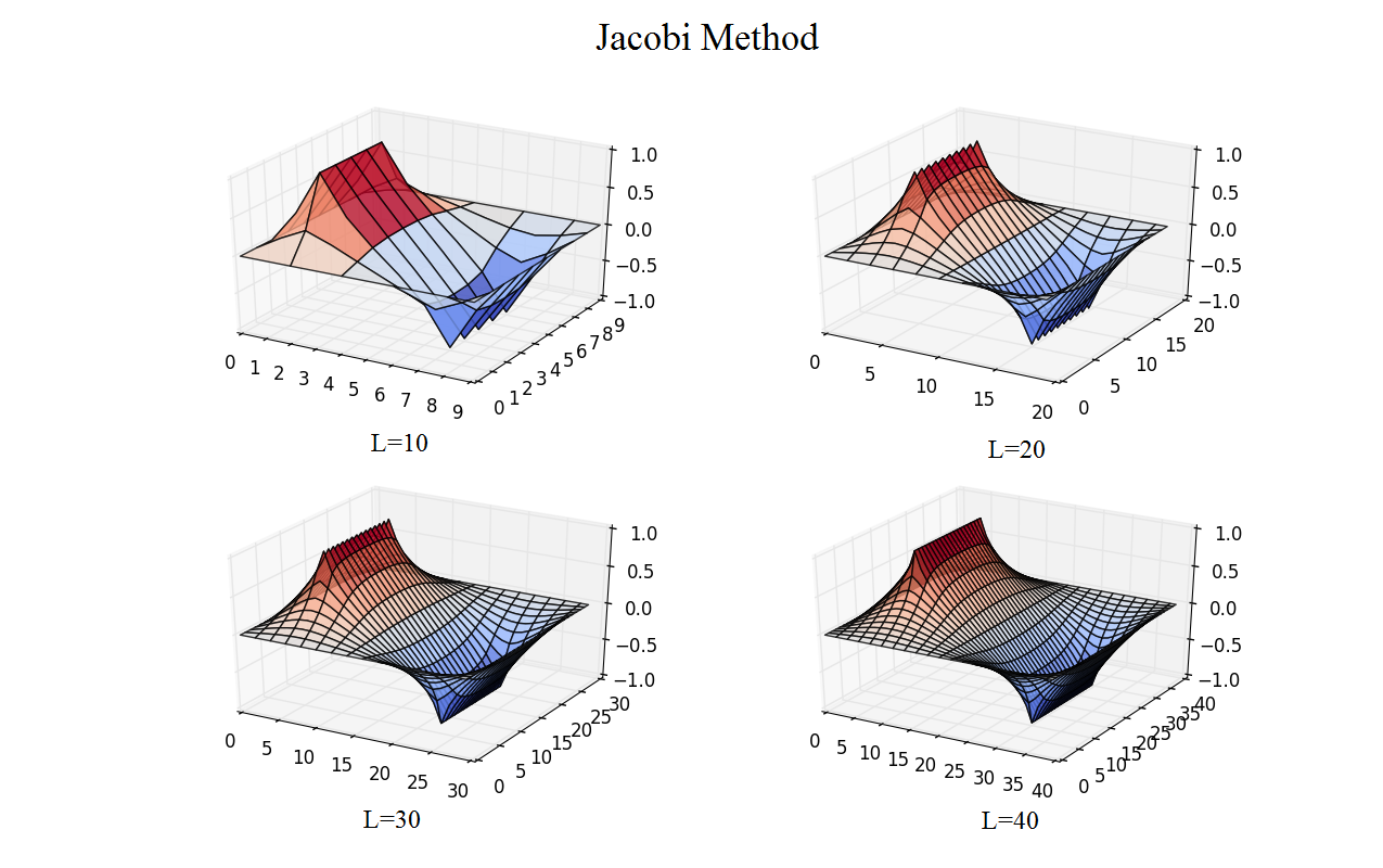
Figure 13.1 Fitting curve of interating time versus time step; the expresssion is given in the figure.
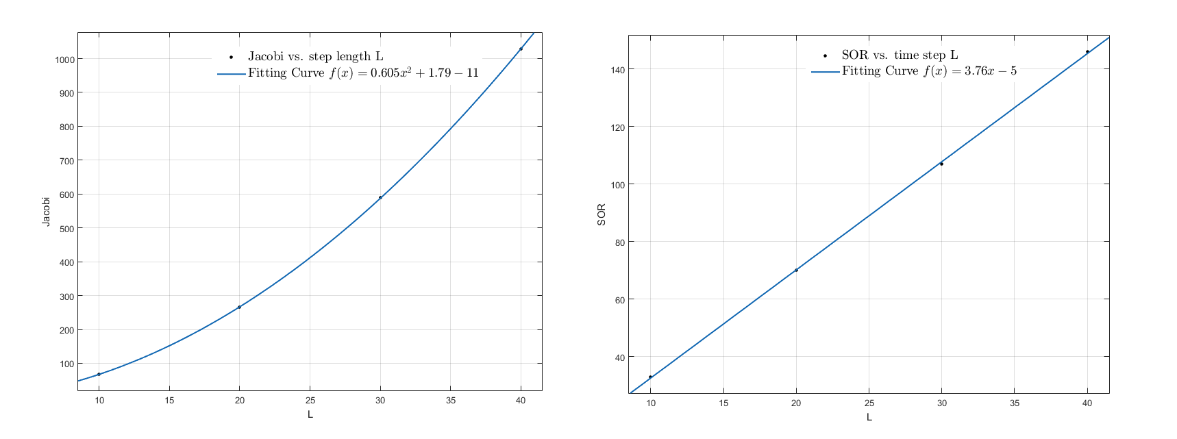
Figure 13.2 Fitting curve of interating time versus time step; the expresssion is given in the figure.
| Step Length | Jacobi Method | SOR method |
|---|---|---|
| 10 | 68 | 33 |
| 20 | 265 | 70 |
| 30 | 589 | 107 |
| 40 | 1028 | 146 |
We used MATLAB to fit the curve with quadrant and linear functions as the result is shown below.
Figure 13.3 Fitting curve of interating time versus time step; the expresssion is given in the figure.
I must devote my appreciation to Li Yao for his code.
-
Giodano, N.J., Nakanishi, H. Computational Physics. Tsinghua University Press, December 2007
-
Jacobi method. (2016, May 16). In Wikipedia, The Free Encyclopedia. Retrieved 12:47, May 22, 2016, from https://en.wikipedia.org/w/index.php?title=Jacobi_method&oldid=720500900
-
Successive over-relaxation. (2016, April 27). In Wikipedia, The Free Encyclopedia. Retrieved 12:46, May 22, 2016, from https://en.wikipedia.org/w/index.php?title=Successive_over-relaxation&oldid=717363228