demo_nn
Demonstrates how to use NeuralNet class for binary classification.
Create XOR dataset
% 2D points in [-1.1,1.1] range with corresponding {-1,+1} labels
m = 400;
X = rand(m,2)*2 - 1;
X = X + sign(X)*0.1;
Y = (prod(X,2) >= 0)*2 - 1;
whos X Y

% shuffle and split into training and test sets
ratio = 0.5;
mTrain = floor(ratio*m);
mTest = m - mTrain;
indTrain = randperm(m);
Xtrain = X(indTrain(1:mTrain),:);
Ytrain = Y(indTrain(1:mTrain));
Xtest = X(indTrain(mTrain+1:end),:);
Ytest = Y(indTrain(mTrain+1:end));
Name Size Bytes Class Attributes
X 400x2 6400 double
Y 400x1 3200 double
Create the neural network
net = NeuralNet2([size(X,2) 4 2 size(Y,2)]);
net.LearningRate = 0.1;
net.RegularizationType = 'L2';
net.RegularizationRate = 0.01;
net.ActivationFunction = 'Tanh';
net.BatchSize = 10;
display(net)
net =
NeuralNet2 with properties:
LearningRate: 0.1000
ActivationFunction: 'Tanh'
RegularizationType: 'L2'
RegularizationRate: 0.0100
BatchSize: 10
% train network
N = 5000; % number of iterations
disp('Training...'); tic
costVal = net.train(Xtrain, Ytrain, N);
toc
% compute predictions
disp('Test...'); tic
predictTrain = sign(net.sim(Xtrain));
predictTest = sign(net.sim(Xtest));
toc
% classification accuracy
fprintf('Final cost after training: %f\n', costVal(end));
fprintf('Train accuracy: %.2f%%\n', 100*sum(predictTrain == Ytrain) / mTrain);
fprintf('Test accuracy: %.2f%%\n', 100*sum(predictTest == Ytest) / mTest);
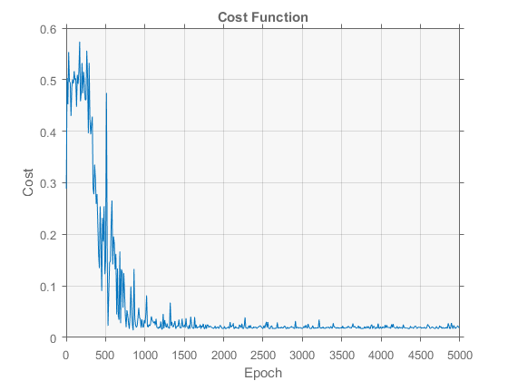
% plot cost function per epoch
figure(1)
plot(1:10:N, costVal(1:10:end)); grid on; box on
title('Cost Function'); xlabel('Epoch'); ylabel('Cost')Training...
Elapsed time is 1.233848 seconds.
Test...
Elapsed time is 0.001355 seconds.
Final cost after training: 0.019445
Train accuracy: 100.00%
Test accuracy: 100.00%
% colors
clr = [0 0.741 0.447; 0.85 0.325 0.098];
cmap = interp1([-1 0 1], ...
    [0.929 0.694 0.125; 1 1 1; 0.494 0.184 0.556], linspace(-1,1,256));

% classification grid over domain of data
[X1,X2] = meshgrid(linspace(-1.2,1.2,100));
out = reshape(net.sim([X1(:) X2(:)]), size(X1));
predictOut = sign(out);

% plot predictions, with decision regions and data points overlayed
figure(2); set(gcf, 'Position',[200 200 560 550])
imagesc(X1(1,:), X2(:,2), out)  % 'CData',predictOut, 'AlphaData',out
set(gca, 'CLim',[-1 1], 'ALim',[-1 1])
colormap(cmap); colorbar
hold on
contour(X1, X2, out, [0 0], 'LineWidth',2, 'Color','k', ...
    'DisplayName','boundaries')
K = [-1 1];
for i=1:numel(K)
    indTrain = (Ytrain == K(i));
    indTest = (Ytest == K(i));
    line(Xtrain(indTrain,1), Xtrain(indTrain,2), 'LineStyle','none', ...
        'Marker','o', 'MarkerSize',6, ...
        'MarkerFaceColor',clr(i,:), 'MarkerEdgeColor','k', ...
        'DisplayName',sprintf('%+d train',K(i)))
    line(Xtest(indTest,1), Xtest(indTest,2), 'LineStyle','none', ...
        'Marker','o', 'MarkerSize',6, ...
        'MarkerFaceColor',brighten(clr(i,:),-0.5), 'MarkerEdgeColor','k', ...
        'DisplayName',sprintf('%+d test',K(i)))
end
hold off; xlabel('X1'); ylabel('X2'); title('XOR dataset')
legend('show', 'Orientation','Horizontal', 'Location','SouthOutside')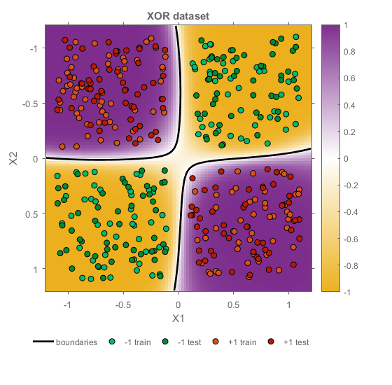
Published with MATLAB R2016a.