MBTI_Classification-

Introduction

Myers–Briggs Type Indicator (MBTI), introduced by Katharine Cook Briggs and her daughter Isabel Briggs Myers is a self-report questionnaire indicating how people with different psychological preferences perceive the world and make decisions. It describes the preferences of an individual using four dimensions of psychological functions which are Extroversion–Introversion (E–I), Sensation–Intuition (S–N), Thinking–Feeling (T–F), and Judgment–Perception (J–P). Also, it can be categorised into 16 categories that includes the combination of the four functions such as ISTJ, ISFJ, INFJ, INTJ and more.

Figure 1 : Eight personality types used in MBTI

Figure 2 : 16 categories of personality type based on MBTI

Example of personality type that corresponds to the text written are: ENTP: “I’m finding the lack of me in these posts very alarming” INFJ: “What? There’s a series! Thanks for letting me know :)”

Objective

The objective of this project is to produce a machine learning algorithm that can attempt to determine a person’s personality type based on some text they have written. We presented two different approaches to tackle this problem. Our algorithm receives text as an input and outputs a predicted MBTI personality type.

Methodology

In this section, we present the visualization of the dataset, the preprocessing steps and model details.

Datasets:

We obtained our data from (MBTI) Myers–Briggs Personality Type Dataset from Kaggle. We visualized the data in figure 3, 4 and 5. From the visualization, the dataset is quite skewed and is not uniformly distributed among the 16 personality types. For example, the most common label, INFP, occurs 1832 times whereas the least frequent, ISFJ, only occurs 42 times. We found that when training on the data in this original form, the model tends to overfit on the predominant type(s) while underperforming on the others.

Data visualization:

The tools that are being used for data visualization are matplotlib, seaborn and word cloud. Figure 3 shows the most occurring words in each category. Figure 4 and figure 5 show the data distribution of the label in the dataset. Figure 4 shows the dataset is actually imbalanced. Figure 5 also shows two classes (each IE, NS) in each label is also imbalanced.

Figure 3 : Common words in each category presented in word cloud

Figure 4 : Frequency of each category

Figure 5 : Frequency of each character in each category

Preprocessing:

Some preprocessing on datasets is necessary. This is because the datasets from Kaggle are collected from users' online forum which are raw and non-formal. The dataset is read using Pandas library. First, every word in the posts is converted to lowercase and all numerics and all links that start with http or https are removed. Then, stopwords are filtered out from the input data to remove words with little meaning. Each word is then lemmatized using WordNetLemmatizer in scikit-learn. To avoid less occurring words or non-english words affect the performance of the model, those words are also removed from the input data.

The two approaches we used required different preprocessing steps. For the first approach, the output from the previous step is feeded into the Bag Of Word (BoW) model, which we used the implementation of CountVectorizer from scikit-learn. Then, term frequency-inverse document frequency (tf-idf) is applied to previous output to obtain a vector representation of each input data point. We used the implementation of TfidfVectorizer from scikit-learn to achieve this. Therefore, we obtained a vector representation for each data point. For the second approach, we create a mapping that maps each word to a unique index. Therefore, the sentences are converted into vector representation.

There are two types of preprocessing for the label for each data point. Both will be evaluated using different models. The first type is each label is encoded into numerical values which range from 0 to 15. Each value represents each label respectively. Figure 6 shows the corresponding value for each label.

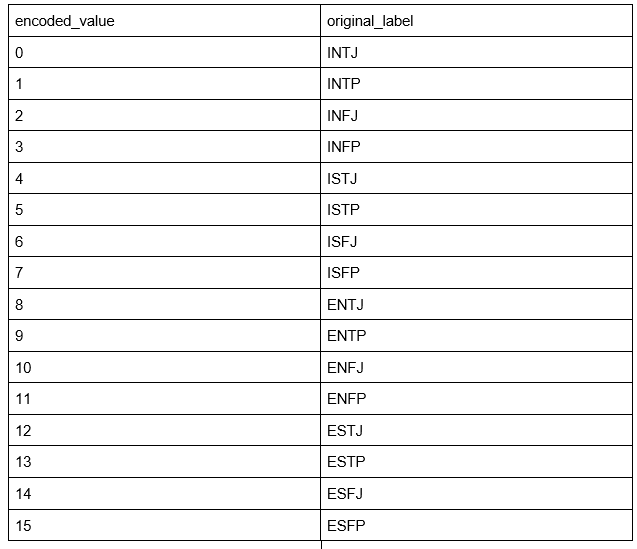Figure 6 : Illustration of first label encoding method

Second type is each character in the label is encoded into 1 and 0 where E=1, I=0 and S=1, N=0 and F=1, T=0 and P=1, J=0. Exact examples that illustrate the result is shown in figure 7.

Figure 7 : Illustration of second label encoding method

The dataset is split into 8:1:1 ratio corresponding to train_size : validation_size : test_size ratio. We utilize the train_test_split function from scikit-learn.model_selection to split the dataset.

Table 1 : Size of each dataset

Model Details:

Model 1 Figure 8 : Model 1 Architecture

In model 1, the target values are all the 16 classes of MBTI types. We used 16 output neurons to represent this. Model 1 consists of 5 hidden layers, which all are fully connected feedforward layers. ReLU activation is added between layer 4 and 5. The output of layer 5 is used as the model's output. Each hidden layer consists of 2000, 750, 250, 50, 16 neurons respectively. We choose Stochastic Gradient Descent (SGD) optimization method to optimize our model based on our chosen objective function Cross Entropy Loss. The learning rate is set to 0.01 and the batch size is set to 100. The model is trained for 300 epochs.

Model 2 Figure 9 : Model 2 Architecture

In model 2, the target value is I or E, N or S, T or F, J or P. We used 4 output neurons to represent this. Each output neuron will give 0 or 1 which indicates the 4 target values respectively. In this model, word embedding is obtained using the embedding layer. Embedded word representation is then passed to LSTM. The last hidden state of LSTM is used as the input of the feed forward layer 1. Output of feed forward layer 1 is passed through ReLU and passed through feed forward layer 2. The output of feed forward layer 2 is used as the model’s output. The embedding dimension is 256, the hidden state dimension of LSTM is 512. We used 1 layer of LSTM in the model. The dimension of the hidden layer is 1024 and 4 respectively. We choose Stochastic Gradient Descent (SGD) optimization method to optimize our model based on our chosen objective function Cross Entropy Loss. The learning rate is set to 0.01 and the batch size is set to 128. The model is trained for 50 epochs.

Results and discussions

According to Table 2, the performance of Model 1 is slightly better in accuracy compared to Model 2. But, Model 2 did better according to F1 score, Recall score and Precision score.

Table 2: Evaluation Result for both model

Suggestions for future work

For future work, we plan to implement a better preprocessing step where we want to convert links into “” token and numerical value to “” token instead of removing it from datasets. Also, we found out that our accuracy is low. That is reasonable because the datasets obtained from Kaggle are imbalanced. Thus, in future we hope to apply a weighted loss function to tackle the disproportion of datasets. We hope to change our optimization method to RMSProp or Adaptive Moment Estimation (Adam) because it nearly always works faster and more reliably while reaching a global minimum and while minimising the cost function. Lastly, we are looking forward to using a more advanced model architecture where we can introduce time steps in data (utilize sequential models such as LSTM).

Part B Processes involved

We include the following flowchart for both approaches showing processes involved to solve the problem of classifying the personality type.

Model 1

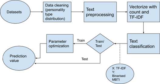
Figure 10 : Flowchart of model 1

Model 2

Figure 11 : Flow chart of model 2

Background theory In this section, we presented the theory of the main algorithm we used in our method.

Bag of Words (BoW) BoW is used to represent text data when modeling text with machine learning. It is a representation of text that describes the occurrence of words within a document. It is called a “bag of words” because it ignores the structure or the order of the words, but only concern with the existence of words. It involves the following steps, with an example of following sentences:

1. Text will be represented as a collection of words.

2. All multiple occurrences of each words are counted and removed while ● Ignoring case ● Ignoring punctuation ● Ignoring frequent words that don’t contain much information, called stop words, like “a,” “of,” etc. ● Fixing misspelled words. ● Reducing words to their stem (e.g. “play” from “playing”) using stemming algorithms.

3. All “word:frequency” from the entire document will be combined creating a vocabulary and will be used to create vectors.

4. Use scoring method to mark the presence of words as a boolean value, 0 for absent and 1 for present, for example text1: “I”=1 “am”=1 “the”=1 “best”=1 “to”=0 ”go”=0 “salad”=0

Text2: “I”=0 “am”=0 “the”=0 “best”=1 “to”=1 ”go”=1 “salad”=1

Now the document is represented in a vector form.

Term Frequency–Inverse Document Frequency (TF–IDF)

TF: It measures how frequent the terms appear in a document. If each document has different length thus the occurrence of words will be different too, whereby a longer document has more terms than shorter document. So, term frequency should be divided by the document length for normalization. The equation as below:

IDF: It is used to rank the importance of a term. In a document, all terms are treated as essential but there are some terms that appear so many times that can be ranked down such as “is”, “a”, “the”. This is because, we want to scale up the scarce words while scale down the frequent words by computing the following:

Fully connected feedforward network

Fully connected feedforward network is made up of multiple layers of perceptrons. Each layer can be defined as

Every hidden layer is connected to its previous layer by a weight . We use feedforward network to map the target value to function of the input value or . The best is obtained using an optimization method.

Long Short-Term Memory (LSTM)

LSTM is a model architecture that extends the concept of recurrent neural network (RNN). It achieved great success in the Natural Language Processing domain by its ability to deal with vanishing and exploding gradient problems. Definition of LSTM is summarized in the figure below.

Figure 12 : LSTM equation

Word Embedding Layer

Word is encoded into dense vector representation in which similar words have similar vector representation. Each word has their own vector representation. This vector representation is learnt during training time.

ReLU Activation

Rectified Linear Unit (ReLU) is a type of non-linear activation function. It is defined as

ReLU is very cheap to compute with the simple equation. It also increases the convergence speed of the model because it does not have a vanishing gradient problem. Since the output of ReLU for all negative values is zero, it produces sparsity within the model. Sparsity often results in less overfitting problems to the model. The model will also be computed faster as there is less calculation to be done.

In our model, ReLU is only used in the hidden layer of the model.

Stochastic Gradient Descent (SGD) Optimization

SGD optimization performs parameters updates for each training example. It is defined as

SGD performs frequent updates with a high variance causing the objective function to fluctuate. This property leads SGD to have potential to escape local minima. However, SGD will overshoot the global minima. Therefore, it is good to slowly reduce the learning rate to achieve convergence.

Cross Entropy Objective Function

We choose to reduce the cross entropy objective function J for optimization.

Experimental protocol We present two different models and compare their performance. We report our performance evaluation on accuracy score, f1 score, precision score and recall score. The metrics are evaluated on the test set. As Table 2 above shows the evaluated result of each model. Figure 13 and figure 14 show the confusion metric on the test set for both models. For model 1, as shown in confusion matrix, the imbalance classes, i.e. I and E, and N and S were misclassified, but the balance classes, i.e. T and F, J and P were well classified. This indicates that once we manage to solve the imbalance class problem, the performance of the model will be improved. This issue also goes to model 2. The class with higher frequency in the dataset gets better prediction while the class with lower frequency in the dataset gets worse prediction.

Figure 13 : Model 1 Confusion Metric on Test Set

Figure 14 : Model 2 Confusion Metric on Test Set

References

1. Mitchelle, J.; Myers-Briggs Personality Type Dataset. Includes a Large Number of People’s MBTI Type and Content Written by Them. Available online: https://www.kaggle.com/datasnaek/mbti-type
2. Uniqtech. (2020, April 23). Understand Cross Entropy Loss in Minutes. Retrieved from https://medium.com/data-science-bootcamp/understand-cross-entropy-loss-in-minutes-9fb263caee9a
3. Sebastian Ruder. (2020, March 20). An overview of gradient descent optimization algorithms. Retrieved from https://ruder.io/optimizing-gradient-descent/index.html#gradientdescentvariants
4. Liu, D. (2017, November 30). A Practical Guide to ReLU. Retrieved from https://medium.com/@danqing/a-practical-guide-to-relu-b83ca804f1f7
5. Olah, C. (2015, August 27). Understanding LSTM Networks. Retrieved from http://colah.github.io/posts/2015-08-Understanding-LSTMs/
6. Gupta, T. (2018, December 16). Deep Learning: Feedforward Neural Network. Retrieved from https://towardsdatascience.com/deep-learning-feedforward-neural-network-26a6705dbdc7
7. Deep Learning: Feedforward Neural Networks Explained. (2019, April 1). Retrieved from https://hackernoon.com/deep-learning-feedforward-neural-networks-explained-c34ae3f084f1
8. Jason B. (2017 October 9) A Gentle Introduction to Bag-of-Words Model. Retrieved from https://machinelearningmastery.com/gentle-introduction-bag-words-model/#:~:text=A%20bag%2Dof%2Dwords%20is,the%20presence%20of%20known%20words.
9. Purva H. (2020 February 28) Quick Introduction to Bag-of-Words (BoW) and Tf-idf for Creating Features from Text. Retrieved from https://www.analyticsvidhya.com/blog/2020/02/quick-introduction-bag-of-words-bow-tf-idf/