GIS

Spatial Skyline Query Problem

Definitions

Concept of Spatial Skyline Queries (SSQ):

• Given a set of data points P and a set of query points Q , each data point has a number of derived spatial attributes (point’s distance to a query point). An SSQ retrieves those points of P which are not dominated by any other point in P considering their derived spatial attributes.
• An interesting variation: an SSQ with the domination is determined with respect to both spatial and non-spatial attributes of P.

Differences between Skyline Queries and Spatial Skyline Queries:

• Spatial skyline points’ distance attributes are dynamically calculated based on the user’s query. The result depends on both data and the given query. Meanwhile skyline points, the result only depends on database.
• The main difference with the regular skyline query is that this spatial domination depends on the location of the query points Q.

Problem illustration:

• Assume that the members of a team located in different (fixed) offices, determine a list of interesting (in terms of traveling distances) restaurants for their weekly meeting lunchs.
• Generating this list becomes more challenging when the team members change location over time.

Formal Problem Definition

General Skyline Queries

Assume that:

• N: number of objects in database (denoted by p).
• p with d real-valued attributes: d-dimensional point $(p_1,..., p_d) \in \mathbb{R}^d$ where $p_i$ is the i-th attribute of p.
• Given the two points $p=(p_1,..., p_d)$ and $p'=(p'_1,..., p'_d)$ in $\mathbb{R}^d$, p dominates p' iff we have $pi \leq p'i$ for $1 \leq i \leq d$ and $p_j < p'_j$ j for some $1 \leq j \leq d$.

Spatial Skyline Queries

Assume that:

• P: set of points in the d-dimensional space. $\mathbb{R}^d$
• D(.,.): distance metric defined in $\mathbb{R}^d$.
• Q={$q_1,..., q_n$}: set of d-dimensional query points.
• Two points p and p' in $\mathbb{R}_d$
• p spatially dominates p' with respect to Q iff we have $D(p, q_i) \leq D(p', q_i)$ for all $q_i \in Q$ and $D(p, q_j) < D(p', q_j)$ for some $q_j \in Q$.

Theoretical Foundation

Concept of Voronoi Diagram, Delaunay Graph, and Convex Hull.

Voronoi Diagram Definition:

• P = ${p_1, p_2,..., p_n}$: set of n distinct points in d-dimensional Euclidean space.
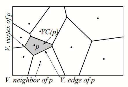
• Voronoi diagram of P: the subdivision of the Euclidean space into n cells, one for each point in P. The cell corresponding to the point $p \in P$ (denoted by VC(p)) contains all the points $x \in \mathbb{R}^d$ s.t $\forall p' \in P, p' \neq p, D(x, p) \leq D(x, p')$.

Note that:

• For Euclidean distance in $\mathbb{R}^2$, VC(p) is a convex polygon.
• Each edge of this polygon (Voronoi edge) is a segment of the perpendicular bisector line of the line segment connecting p to another point of the set P.
• Each Voronoi edge of the point p refers to the corresponding point in the set P as a Voronoi neighbor of p.

Delaunay Triangulation and Delaunay Graph Definition.

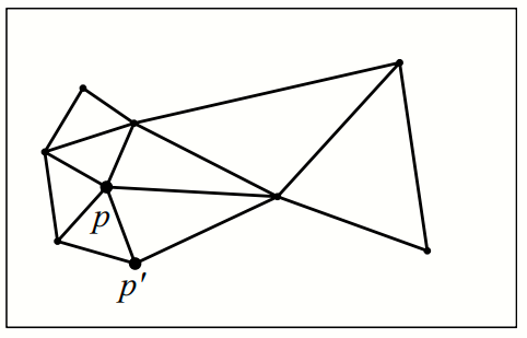
• Delaunay Triangulation is a triangulation of a set of points P such that the circumcircle of each triangle contains no other points in its interior.
• It maximizes the minimum angle of the triangles and minimizes the maximum circumradius of the triangles.
• The Delaunay Graph can be obtained from the Delaunay Triangulation.

Convex Hull Definition.

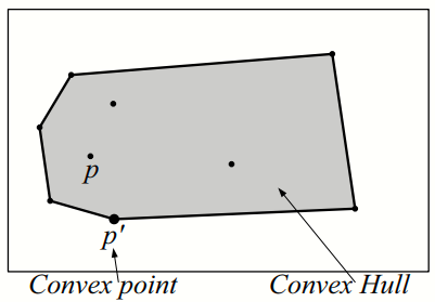
• The Convex Hull (CH(P)) of points in $P \subset \mathbb{R}^d$, is the unique smallest convex polytope (polygon when d = 2) which contains all the points in P.
• $CH_v(P)$ is the set of CH(P)'s vertices, called convex points. All other points in P are non-convex points.
• The shape of the Convex Hull of a set P only depends on the convex points in P.

Theories.

We use lemma (1) and two theorems 1 and 3 to identify definite skyline points and theorem (2) to eliminate query points not contributing to the search.

• Lemma 1: For each $q_i \in Q$, the closest point to $q_i$ in P is a skyline point.
• Theorem 1: Any point $p \in P$ which is inside the convex hull of Q is a skyline point.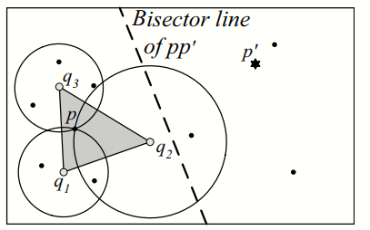
  
• Lemma 2: Given two query sets $Q' \subset Q$, if a point $p \in P$ is a skyline point with respect to Q', then p is also a skyline point with respect to Q.
• Theorem 2: The set of skyline points of P does \textit{not depend} on any non-convex query point $q \in Q$.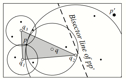
  
• Theorem 3: Any point $p \in P$ whose Voronoi cell V C(p) intersects with the boundaries of convex hull of Q is a skyline point.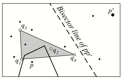
  

Solutions

Static Queries

Branch-and-Bound Spatial Skyline Algorithm ($B^2S^2$).

Asume that:

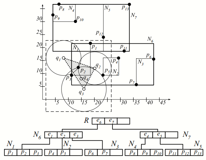
• The data points are indexed by a data-partitioning method such as R-tree.
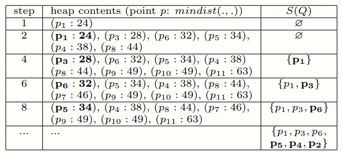
• mindist(p, A): be the sum of distances between p and the points in the set A ($\Sigma _{q \in A} D(p, q)$).
• mindist(e, A): as the sum of minimum distances between the rectangle e and the points of A ($\Sigma _{q \in A} mindist(e, q)$)
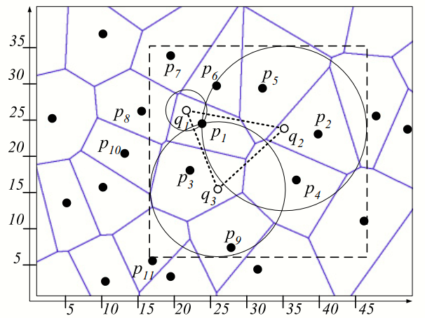
• Data points P = {p1,..., p13} and query points Q = {q1,..., q4}.

Steps:

• Step 1: Compute the convex hull of Q and determines the set of its vertices CHv(Q).
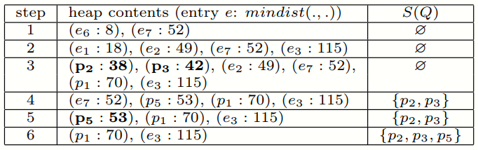
• Step 2: traverse the R-tree and maintaining the minheap H sorted based on the mindist values of the visited nodes.

For example:

Voronoi-based Spatial Skyline Algorithm ($VS^2$).

Ideal:

• VS2 algorithm uses the Voronoi diagram (the corresponding Delaunay graph) of the data points.
• R-tree on the data points does not exist.
• The points whose Voronoi cells are inside or intersect with the convex hull of the query points are skyline points.
• The adjacency list of the Delaunay graph is stored according to points' Hilbert values.

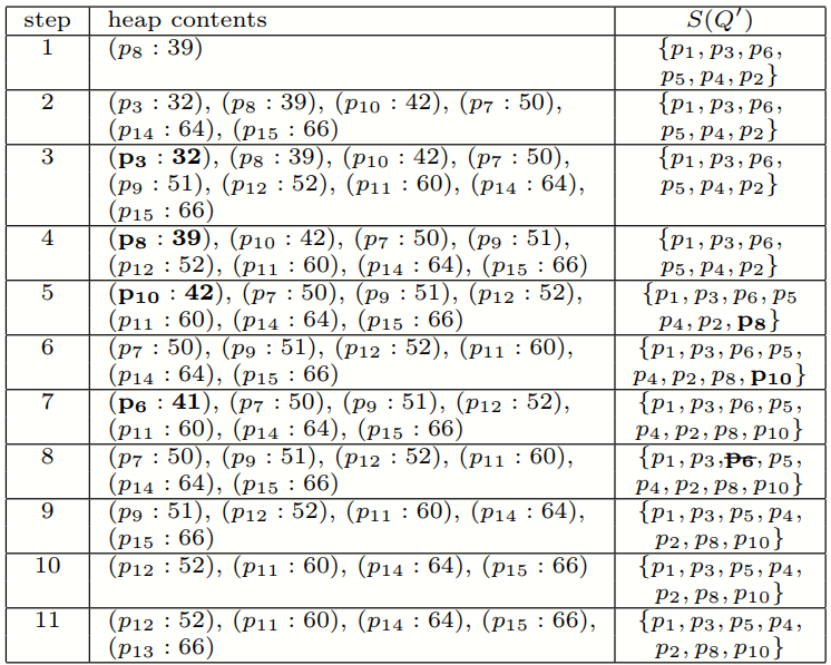
Steps:

• Traverse the Delaunay graph starting from the closest point to a query point and determining traversal order based on a monotone function $mindist(p,CH_v(Q))$.
• Maintain two lists of visited and extracted points and a rectangle B of candidate skyline points.
• Add the closest point to the heap and iteratively examines the top entry.
• Add skyline points if they are not dominated by current skyline and updates Extracted and B.
• Add unvisited Voronoi neighbors to Visited and Heap if conditions are met.
• Return the skyline points when the heap becomes empty.

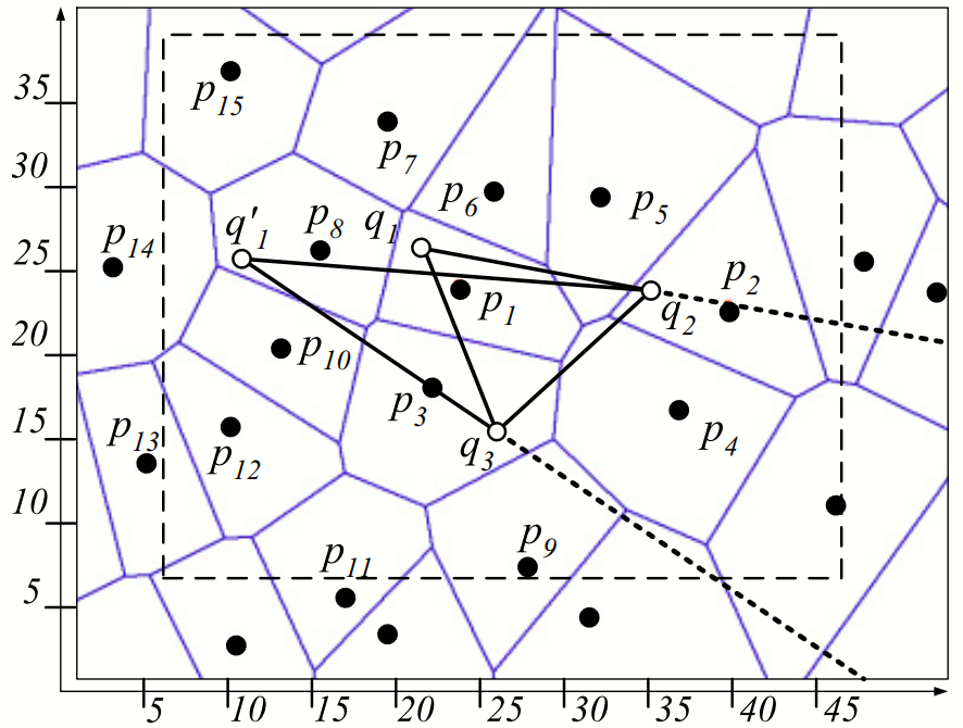
For example:

Continuous Queries

What happens whenmquery points change their locations?

• Recompute spatial skyline points.
• Problem: R-tree-based algorithms (B2S2 and BBS) are expensive because the entire R-tree must be traversed per each update.
• Solution: update the set of previously found skyline points by examining only those data points which may change the spatial skyline.
• Idea:
  • Find the query points which may change the dominance of a data point outside CH(Q). (Lemma 4)
  • Choose the data points that must be examined when the location of q changes. (Lemma 5)

Assume that:

• $CH_v^+(Q)$ and $CH_v^-(Q)$: sets of the vertices on the closer and farther hulls of the convex hull CH(Q) to p, respectively.

• Lemma 4: Given a data point p and a query set Q, the dominance of p only depends on the query points in $CH_v^+(Q)$.

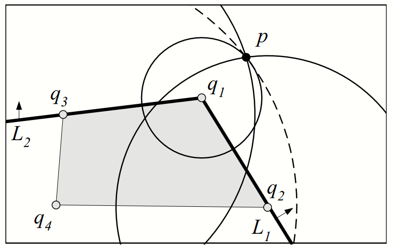
• Lemma 5: The locus of data points whose dominance depends on $q \in CH_v(Q)$ is the visible region of q.

For example:
$\rightarrow$ $CH_v^+(Q) = {q_1, q_2, q_3}$ and $CH^-_v(Q) = {q_4}$.

Voronoi-based Continuous SSQ ($VCS^2$).

Assume that:

• q’ :new location of q
• Q’ = $Q\cup {q’}- {q}$ new set of query locations.

Steps:

• Compute the convex hull of the latest query set CH(Q’).
• Compares CH(Q’) with the old convex hull CH(Q).
• Depending on how CH(Q’) differs from CH(Q), $VCS^2$ decides to:
  • Case 1: traverse only specific portions of the graph and update the old skyline S(Q).
  • Case 2: rerun $VS^2$ and generate a new one.
• Retrieve points in the candidate area and update Skyline S(Q) for new points.
• Removes inverted points from Skyline S(Q).

Case 1: Situations where VCS2 updates the skyline based on the change in CH(Q’).

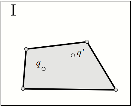
Pattern I: CH(Q) and CH(q’) are identical, the skyline does not change and no graph traversal is required. (Theorem 2)

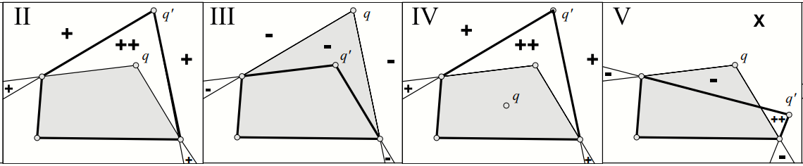
Patterns II-V: The intersection region of CH(Q) and CH(Q’) skyline points to both Q and Q’, no traversal needed.

• The region "++": points inside CH(Q’) and outside CH(Q). Any point in this region is a skyline point with respect to Q' $\rightarrow$ add to the skyline. (Theorem 1)
• The region "+": points whose dominator regions have become smaller $\rightarrow$ might be skyline points and must be examined.
• The region "-": points whose dominator regions have been expanded $\rightarrow$ delete from the old skyline.
• The regions "x": must be examined as their dominator regions have changed.
• Unlabeled white region: points outside of the visible regions of both q and q’ $\rightarrow$ remain the same. (Lemma 5)

For example:

Experiment

Branch-and-Bound Spatial Skyline Algorithm ($B^2S^2$).

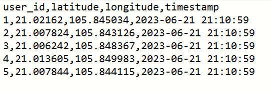
Dataset of 5 query points.

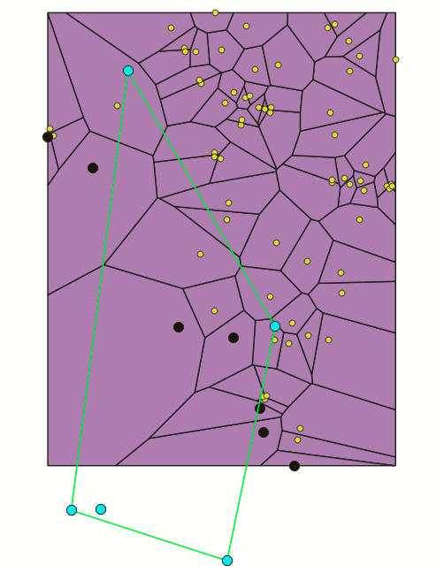
Green polygon: convex hull of Q.
Yellow points: locations of restaurant (OpenStreetMap).
Black points: Spatial Skyline points.

Voronoi-based Spatial Skyline Algorithm ($VS^2$).

Dataset of 5 query points.

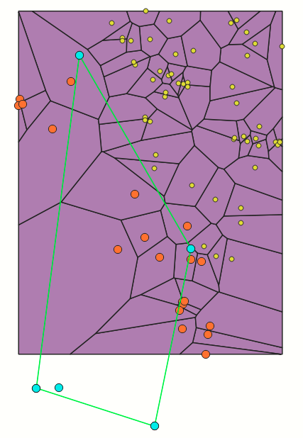
Green polygon: convex hull of Q.
Yellow points: locations of restaurant (OpenStreetMap).
Orange points: Spatial Skyline points.

Voronoi-based Continuous SSQ ($VCS^2$).

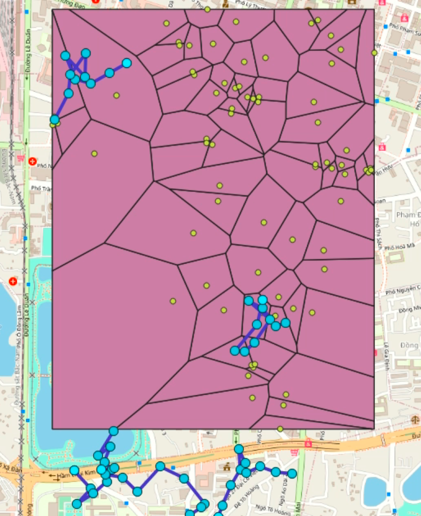
Dataset of 5 query points.

To run this project

• Use anaconda to create python environment:

  • conda create --name yourname python=3.8
  • conda activate yourname

• Install Pycharm (suggestions>=3.7) and related environmental dependencies:

  pip install -r requirements.txt

• Extract spatial data from openstreetmap.org.

• Visualize on Qgis.

Citation

[Mehdi Sharifzadeh and Cyrus Shahabi. The Spatial Skyline Queries.]