Home
YANG-DB is a graph query engine. It is based on elasticsearch as the physical graph storage layer and the tinkerpop graph traversing framework.
- Versatile Engine API including query cursor and paging
- Pattern based graph query language [Cypher] (https://opencypher.org/)
- Cost based optimizer to enable fast and efficient graph search
- Customized graph schema definition and enforcement
-
Installation tutorial: https://github.com/YANG-DB/yang-db/blob/develop/docs/tutorial/sample/dragons/installation.md
-
Schema creation tutorial: https://github.com/YANG-DB/yang-db/blob/develop/docs/tutorial/sample/dragons/create-ontology.md
-
Data Loading tutorial: https://github.com/YANG-DB/yang-db/blob/develop/docs/tutorial/sample/dragons/load-data.md
-
Query the Graph tutorial: https://github.com/YANG-DB/yang-db/blob/develop/docs/tutorial/sample/dragons/query-the-data.md
-
Projection materialization & count tutorial: https://github.com/YANG-DB/yang-db/blob/develop/docs/tutorial/sample/dragons/projection-and-count.md
The Process of transforming the Cypher into the physical layer traversal and execution of the query is composed of the several phases, each has a distinct purpose
- ASG – Abstract Syntax Graph (also known as Abstract Syntax Tree )
- EPB – (Logical) Execution Plan Builder
- GTA – Gremlin Traversal Appender (Physical Plan Builder)
- Executor – Executed the Physical Plan
- Results projector – Projects the results back to logical
We are using a proprietary intermediate Graph traversal language
This is a logical high-level (property) graph query language which has an emphasize on query patterns, and visual attributes.
“It is a declarative visual query language for schema-based property graphs.
It supports property graphs with mixed (both directed and undirected) edges and half-edges, with enumerated, multivalued and composite properties, and with empty property values.
It supports temporal data types, operators, and functions, and can be extended to support additional data types, operators, and functions (one spatiotemporal model is presented)…”
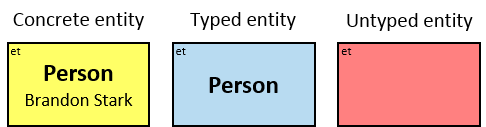
A node can be one of the next:
- CONCRETE ENTITY – Specific entity in the graph
- TYPED ENTITY – A subclass of typed entity category / categories
- UNTYPED ENTITY – Entity of Un specified type
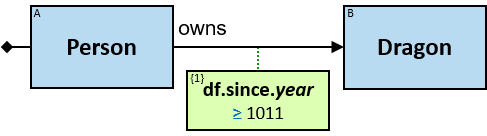
A logical relationship type is defined by a pattern:
- Two typed/untyped entities in the pattern
- A relationship type name assigned to each such relationship
- A logical relationship type can be either directional or bidirectional.
A filter on entities or relationships which refer to non-concrete entities.

Our internal language supports the following primitive data types:
- Integer types
- Real types (floating-point)
- String
- Date
- datetime
- duration
- Quantifier can be used when there is a need to satisfy more than one constraint.
- Quantifier can combine both constraints and relations
Start – The query start node
####Entities Entity can belong to one of the next categories:
- EUntyped – Untyped Entity
- ETyped –Typed Entity
- Has list of possible types
- EConcrete – Concrete Entity Type
- Has a concrete id
####Relationships Relationship has direction & type (Can support untyped relations)
- Rel – Relationship
####Properties Every relation & entity can have properties.
- RelProp – Relationship property
- EProp – Entity property
Properties have name, type (data type) & constraint:
- RelPropGroup – Relationship property group
- EPropGroup – Entity property group
####Constraint
Constraint is combined of an operator and an expression.
A constraint filters assignment to only those assignments for which the value of the expression for the assigned entity/relationship satisfies the constraint.
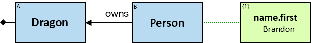
Query as a json document:
{
  "name": "Q1",
  "elements": [
    {
      "eNum": 0,
      "type": "",
      "next": 1
    },
    {
      "eNum": 1,
      "type": "EConcrete",
      "eTag": "A",
      "eID": "12345678",
      "eType": "Person",
      "eName": "Brandon Stark",
      "next": 2
    },
    {
      "eNum": 2,
      "type": "Rel",
      "rType": "own",
      "dir": "R",
      "next": 3
    },
    {
      "eNum": 3,
      "type": "ETyped",
      "eTag": "B",
      "eType": "Dragon"
    }
  ]
}
Additional simple string representation:
Start [0]: EConcrete [1]: Rel [2]: ETyped [3]Each query has a name and a (linked) list of elements which are labeled with :
- eNum - sequence number
- eTag – a named tag used for results labeling
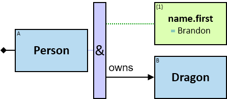
Additional Query with quantifier and property constraint
{
  "name": "Q10",
  "elements": [
    {
      "eNum": 0,
      "type": "Start",
      "next": 1
    },
    {
      "eNum": 1,
      "type": "ETyped",
      "eTag": "A",
      "eType": "Person",
      "next": 2
    },
    {
      "eNum": 2,
      "type": "Quant1",
      "qType": "all",
      "next": [
        3,
        4
      ]
    },
    {
      "eNum": 3,
      "type": "EProp",
      "pType": 1,
      "pTag": 1,
      "con": {
        "op": "eq",
        "expr": "Brandon"
      }
    },
    {
      "eNum": 4,
      "type": "Rel",
      "eType": "own",
      "dir": "R",
      "next": 5
    },
    {
      "eNum": 5,
      "type": "ETyped",
      "eTag": "B",
      "eType": "Dragon",
      "next": 6
    }]
}
Additional simple string representation:
Start [0]: ETyped [1]: Quant1 [2]:{3|4}: EProp [3]: Rel [4]: ETyped [5]Start node – is the query begin element, each query element number appears in the rectangle brackets. Quantifiers sub-elements appear in the curly brackets. ##ASG - Abstract Syntax Graph
In the process of receiving the graph query we want to apply a set of predefined simple strategies that would transform the logical query to a lower lever logical query.
Performing:
- Query Validation
- Grouping of similar attributes (transform eProp’s into ePropGroup)
- Infer untyped expressions
- Constraints transformations (String to concrete types)
####Validity A query is considered valid when it preserves the traversal steps:
- (Entity | optional costraints)-[Relation|optional costraints]->(Entity)
- (Entity | optional costraints)-{Quantifier}-R(i):[Relation]|optional costraints]->(Entity)
Another validation concern is the constraints of the graph’s schema;
An entity may by of a given type A which has properties a1 & a2. If constraint exists in the query, it must follow the entity's properties.
##(L)EPB - Logical Execution Plan Builder

The responsibility of this phase is to transform (build) ASG query into a plan which is cost optimized according to set of predefined statistical parameters collected over the dataset.
###Strategies The Logical Plan executor is responsible for building a valid (logical) execution plan that will later be translated into physical traversal execution plan.
The Plan Execution Builder comes with 3 strategies:
-
DFS – A simple (DFS based) strategy that uses regular extenders to build the plan without any cost estimation.
- Extenders will try depth first (descendants) strategy for plan building.
-
Rule Based – A simple strategy that uses regular extenders to build the plan without any cost estimation.
- Extenders will attempt to select ‘low cost’ steps according to some predefined simple rules.
-
Cost Based – Cost based plan builder will use regular extenders with an additional cost estimation step.
- Extenders are more exhaustive then in the former plans to cover as many plans as possible.
- Cost estimation will be used to prune costly plans.
The EPB process essentially is constantly growing a logical execution plan using the next components
- Extenders – add steps to existing plan in a variety of manners
- Pruners – remove plans either not valid or not efficient or duplicate
- Selector – selects best plans to continue to groom
- Statistics – provides the statistical cost access above the dataset
- Estimator – calculation the additional step cost according to the statistics
The extending phase is somewhat exhaustive in the way it adds steps to the plan.
This is useful in overcoming local minimums, the downside is the size of the plans search tree, we employ the pruner (for the purpose of trimming the tree size). The pruner acts according to size & cost minimization – for example we only allow plan with 3 joins at most (this is configurable).
Only the cost based strategy will employ cost based selectors & pruners.

####Initial Extenders
Initially we begin with empty plan and spawn initials (single step) plans, all plans start from ETyped node. We continue the process of plan building with the next steps...
While we have available search options (unvisited query elements) do:
- Extend plan with a single step (apply a series of extenders)
- Each (next) step is taken from the query unvisited elements.
- Validate the extended plan (apply a series of validators)
- Estimate cost for each plan (add the cost of the latest step)
- Select (Prune) best plan according selector policy (lowest cost / size limitation and so on… )
Once no more new steps available – we should have a list of valid best prices plans of which we will take the first (or any) for execution.
####On-Going Extender Types An extender attempts to extend an existing plan with the next patterns:
(entity)—[relation]—(entity) (entity):{constraints}—[ relation] :{constraints}—(entity) :{constraints} (entity)—[relation]—(entity)—(goTo:visited_entity)
From any step in the execution plan, we try to extend the plan either left or right (with elements from the query) Left is considered ancestor, right is considered descendant.
####Example 1
Let’s assume we have the next query:
Start [0]: ETyped [1]: Quant1 [2]:{3|4}: EProp [3]: Rel [4]: ETyped [5]• ETyped [1] – Plan 1
• ETyped [5] – Plan 2Next, we need to add additional steps (from the query) which are not part of the plan
- Extending each plan with all possible extenders (all directions)
StepAncestorAdjacentStrategy – extender that attempts extending left (ancestor)
• ETyped [1] (no left extension possible) – Plan 1
• ETyped [5] --> Rel[4] --> ETyped [1]:EProp[3] – Plan (2)-3
StepDescendantsAdjacentStrategy –extender that attempts extending right(Descendant)
• ETyped [5] (no right extension possible) – Plan 2
• ETyped [1]: EProp [3] --> Rel [4] --> ETyped [5] – Plan (1)-4The final plans are 3 & 4, there are similar but in reverse order.
####Example 2 Additional available Extender strategies... Let’s assume we have the next query:
Start [0]: ETyped [1]: Quant1 [2]:{3|4|6}: EProp [3]: Rel [4]: ETyped [5] : Rel [6]: EConcrete[7]First Phase:
•	ETyped [1] – Plan 1
•	ETyped [5] – Plan 2
• ETyped [7] – Plan 3Second Phase: Extending each plan with all possible extenders (all directions)
StepAncestorAdjacentStrategy – extender that attempts extending left (ancestor)
• ETyped [1] (no left extension possible) – Plan 1
• ETyped [5] --> Rel[4] --> ETyped [1]:EProp[3] – Plan (2)-4
• ETyped [7] --> Rel[6] --> ETyped [5] - Plan (3)-5
StepDescendantsAdjacentStrategy –extender that attempts extending right(Descendant)
• ETyped [7] (no right extension possible) – Plan 3
• ETyped [5] --> Rel[6] --> ETyped [7] – Plan (2)-5
• ETyped [1]:EProp[3] --> Rel [4]-->ETyped [5] – Plan (1)-6
GotoExtensionStrategy - extender that jumps to already visited element
• ETyped [5]-->Rel[4]--> ETyped [1]:EProp[3]-> GoTo[5] – Plan (4)-7
• ETyped [1]:EProp[3]--> Rel[4]--> ETyped[5]-> GoTo[1] – Plan (6)-8
• ETyped [5] --> Rel[6] --> ETyped [7]-> GoTo[5] - plan (5)-9Forth Phase:
StepAncestorAdjacentStrategy – extender that attempts extending left (ancestor)
• ETyped[7]-->Rel[6]-->ETyped[5]-->Rel[4]-->ETyped[1]:EProp[3] - Plan (5)-10
• ETyped[5]-->Rel[6]-->ETyped[7]->GoTo[5]-->Rel[4]-->ETyped[1]:EProp[3] – plan (9)-11
StepDescendantsAdjacentStrategy –extender that attempts extending right(Descendant)
• ETyped[1]:EProp[3]-->Rel[4]-->ETyped[5]-->Rel[6]->EConcrete[7] – Plan (5)-12
• ETyped[5]->Rel[4]->ETyped[1]:EProp[3]->GoTo[5]-->Rel[6]->EConcrete[7] – Plan (8)-13Plans 10-13 are the final plans, while additional non-valid plans had been removed during the build process. The missing step here is the cost estimation. In the next section we will apply the same plan building process but with the additional cost estimators.
####Example 3
Examining the Join Extender... Let’s assume we have the next query:
Start [0]: ETyped [1]: Quant1 [2]:{3|4|6}: EProp [3]: Rel [4]: ETyped [5] : Rel [6]: EConcrete[7]First Phase:
•	ETyped [1] – Plan 1
•	ETyped [5] – Plan 2
•	ETyped [7] – Plan 3
Second Phase: Todo ...
##Cost Estimator

Cost estimator is the process of evaluating a “cost” of an execution plan according to a prior made statistical calculation for the distribution of values in the dataset.
Each execution step (element in the query) of any graph element (entity, relation, filter) will be estimated based on the physical storage statistical attributes of the data.
####Redundancy Redundancy is the process of pushing node attributes to adjacent relations – making them redundant in the data. The purpose of this process will increase the volume of data stored on one hand, on the other hand it will decrease
the amount of data needed to fetch in each query, and will enable more accurate execution plan. In a redundant model we will store on each relation both id’s of the relating sides, the relating types and any of the sides properties we may think may be of redundancy value.
####Collecting statistical data process

The process of collecting statistical information about elements of the graph – is tightly connected to the physical storage format of the underlying DB.
In a non-native graph DB that its storage mechanism is based on a document store. The graph elements – both node & edges are stored in a document. we need to calculate the histogram (distribution) for every property in the graph.
In a document store like elasticsearch there is an additional level of abstraction for the document location and partitioning:
-
Indices – indicate the “table” (index) that holds all the “records” of a given type
-
Shard – The table’s (index) “partition” factor that partitions the data according to some column (mostly time based)
-
Mappings – mappings is Elasticsearch’s schema index structure, we use it to label the graph elements with a distinct type (each type can have named properties).
###Types of statistical estimators:
Histogram with buckets (bucket per schema type)
- Each bucket contains:
- Cardinality of entity types
- Document count for entity types
Histogram with buckets (bucket per range)
- Each bucket contains:
-
- Field cardinality
-
- Graph elements cardinality
####Graph element properties Example Let’s assume we have a Person entity type with name property, we will create a histogram with 26 buckets – one per each starting letter.
Given a bucket for the letter ‘J’ – it will contain the unique name (starting with J) in the data (Jack, Jhon) and the unique Entities with that name.
We can observe that the entity cardinality (unique people with names starting with ‘j’) for that bucked would be much higher than of the value cardinality (unique names starting with ‘j’) since many person entities can share the same name.
Estimating the number of People named ‘James’ would take us to the next formula: ‘J’-Bucket cardinality: [100, 350000] – 100 stands for unique names starting with J and 350,000 stands for unique people with names starting with J. Estimate will be 350,000 / 100 = 35000. Let’s assume we would like to estimate number of people named ‘JMorgam’ –
If we assume equal distribution of cardinality inside the bucket, we may take the assumption that since the second letter is M - which is about in the middle of the alphabet, we can get better estimation by assuming ½ of the values are from the letter ‘m’ onwards ... Estimate will be (350,000 / 100) /2 = 17500.
####Bucket Ranges – depends on field type Bucket may have the following ranges (according to the field type)
Numeric – given bucket number and min-max range – buckets range according to data
String - alphabetic range buckets (equal width / depth)
Manual - manual number & size buckets (user defined)
Term - buckets stands for a string term according to number of terms in the data
Dynamic – given bucket number, auto calculate min-max (numeric only) according to data
####Relation – Let’s review relation histogram; The histogram is defined to measures count & cardinality of the following tuple
(A,B are the relations side respectively) :
{A.id, A type, B.id, B type, Rel.id, direction, values}.Each relation type (owns, lives, knows...) will have this histogram, the number of buckets will be the cartesian product of the tuple elements (assuming non-valid combinations such as ‘car-[owns]->person’ is not allowed)
Each of these buckets will contain:
- Count of relations id’s
- Count of SideA unique entities
- Cardinality of SideA
Let’s assume we have 10 entity types, then the number of buckets will be: Side A - 10 (possible types) X Side B - 20 (possible types) X2 (directions) = 400.
Owns – 3 dimensional histogram for ‘own type relation.
{
  "type": "owns",
  "fields": [
    {
      "field": "entityA.type",
      "histogram": {
        "histogramType": "manual",
        "dataType": "term",
        "buckets": […]
      }]
    },
    {
      "field": "entityB.type",
      "histogram": {
        "histogramType": "manual",
        "dataType": "term",
        "buckets": […]
    },
    {
      "field": "dir",
      "histogram": {
        "histogramType": "manual",
        "dataType": "term",
        "buckets": […]
       }
    }
  ]
}
##Filter selectivity – A filter condition is a predicate expression specified in the predicate clause (property constraint) of a query.
A predicate can be a compound logical expression with logical AND, OR, NOT operators combining multiple single conditions.
A single condition usually has comparison operators such as =, <, <=, >, >= or <=>2.
For logical AND expression, its filter selectivity is the selectivity of left condition multiplied by the selectivity of the right condition:
selectivity(a AND b) = selectivity(a) * selectivity(b).
•	empty
•	notEmpty
•	eq
•	ne
•	gt
•	ge
•	lt
•	le
•	inset
•	notInSet
•	inRange
•	notInRange
•	contains
•	notContains
•	startsWith
•	notStartsWith
•	endsWith
•	notEndsWith
•	match
•	notMatch
•	fuzzyEq
•	fuzzyNe
##Collection Statistics Framework
For every property we collect histogram data, each histogram has a list of buckets holding monotonic range of content, the location of its content (index, shard) type, documents count & cardinality.
###Example fields to histogram mapping The next example has 3 types of histograms for 3 fields:
- Age – numeric histogram
- Name – String histogram (equal width bucket size)
- Address – manual buckets histogram
"types": [{
  "type": "dragon", #(entity type)
  "fields": [{
    "field": "age", #(field name)
    "histogram": {
      "histogramType": "numeric",
      "min": 10,
      "max": 100,
      "numOfBins": 10
    } },
    {
      "field": "name",
      "histogram":
      {
        "histogramType": "string",
        "prefixSize": 3,
        "interval":10,
        "firstCharCode":"97",
        "numOfChars":26
      } },
    {
      "field": "address",
      "histogram":      {
        "histogramType": "manual",
        "dataType":"string",
        "buckets":[
          { "start":"abc",
            "end": "dzz"
          },
          { "start":"efg",
            "end": "hij"
          },
          { "start":"klm",
            "end": "xyz"
          }]
	}
    }]
String histogram:
numOfBuckets = Math.ceil(Math.pow(numChars, prefixLen) / interval##Join In relational algebra join has 4 type semantics:
- Inner join
- Left outer join
- Right outer join
- Full outer join
In the graph semantics, traversing from node a -> b is performing inner join between a type elements and b type elements, fetching only the (a,b) records that have relationship.
Left & right outer joins (Right outer join) in graph semantics are equivalent to optional graph operators. Optional operator a --Optional-->b will fetch all type of a’s and if exists relation to b’s it will also bring them.
The direction of the join is according to the direction of the relation.
###Join cost estimation
For estimating the join cost we currently assume using in memory hash-join; lets assume we need to join two groups A with size n and B with size m. The cost of doing in-memory hash join is the I/O cost of fetching the groups from the data-set to the driver,
cost = O(m) + O(n). The count estimation of the elements after the join is the smallest size group docCount = min(docCount(m),docCount(n))
This is an upper bound estimation; the actual count may be lower.
###Cost Estimator is Pattern Based For an existing plan, adding a step to the plan has a price, this price is added to the current total price of the plan.
Cost is estimated for the following steps:
EntityPattern – EntityPatternCostEstimator cost estimatorEstimates single entity step cost – entity docCount (with filter if exists)
EntityRelationEntityPattern – EntityRelationEntityPatternCostEstimator cost estimatorEstimates (entity)-->[relation]-->(entity) step cost – see formula below
GoToEntityRelationEntityPattern – GoToEntityRelationEntityPatternCostEstimator cost estimatorEstimates cost of the entity relation entity pattern with additional goTo step
We will use the next schema: ###Entities: Person (1M distinct values)
-
id
-
Name (1K distinct values)
-
- String Histogram with about 2000 buckets (equal width)
-
Age (100 distinct values)
-
- Dynamic Histogram with 100 buckets
-
- Gaussian age distribution (mean = 25)
-
Gender
-
- Term Histogram with 2 buckets, 50% in each bucket
City (500 distinct values)
- Name
-
- Term Histogram with about 500 buckets (number of distinct models)
- Country (50 distinct values)
-
- Term Histogram with about 50 buckets (number of distinct models)
Car (100 distinct values)
- Brand
-
- Term Histogram with 100 buckets (number of distinct models)
Company (1000 distinct values)
- Name
###Relations: Owns (Person->car)
- 50% of the people own car (geometric distribution with mean 1)
Time of purchase - (10K distinct values)
-
- Dynamic Histogram with 100 buckets
Selectivity: (average number of edges)
-
- Number of Persons / Number of distinct edges
Collision Factor:
-
- Number of Edges / Number of distinct Cars
Redundant Properties Holds count & cardinality of the edges within the context of the measured redundant property.
####Side A
-
- Person Name – multidimension histogram [name, direction]
-
-
- String Histogram with about 2000 buckets (equal width)
-
-
- Person age – multidimension histogram [age, direction]
-
-
- Dynamic Histogram with 100 buckets
-
####Side B
-
- City Name – multidimension histogram [name, direction]
-
-
- Term Histogram with about 500 buckets (number of distinct models)
-
-
- City Country – multidimension histogram [country, direction]
-
-
- Term Histogram with about 50 buckets (number of distinct models)
-
####Located-In (Person->City, Company->City)
Selectivity: (average number of edges)
- [Person, City]: Number of Persons / Number of (Unique Person) Located-In edges
- [Company, City]: Number of Company / Number of (Unique Company) Located-In edges
Collision Factor:
- Number of Persons / Number of Cities
- Number of Companies / Number of Cities
####Redundant Properties [Person,City]
Side A
- Person Name – multidimension histogram [name, direction]
-
- String Histogram with about 2000 buckets (equal width)
-
- 262626 / 10 = 26^prefixSize / interval
- Person age – multidimension histogram [age, direction]
-
- Dynamic Histogram with 100 buckets
Side B
- City Name – multidimension histogram [name, direction]
-
- Term Histogram with about 500 buckets (number of distinct models)
- City Country – multidimension histogram [country, direction]
-
- Term Histogram with about 50 buckets (number of distinct models)
[Company,City]
Side A
- Company Name – multidimension histogram [name, direction]
Side B
- City Name – multidimension histogram [name, direction]
-
- Term Histogram with about 500 buckets (number of distinct models)
- City Country – multidimension histogram [country, direction]
-
- Term Histogram with about 50 buckets (number of distinct models)
Friend (Person->Person)
- todo
Works (Person->Company)
- todo
##Query
Person[1]:Quant1[2]:{3|4|6}:Person.name[3]{start with “dan”}:Owns[4]:Car[5]:located[6]:City[7]: City.name[7]{equals “N.Y”}This query will be estimated on each step the extender adds, lets start the process by applying the initial extender & evaluating cost according to type’s count & cardinality
Phase 1: (Initial Extender)
EType[1]: EProp[3] - cost : (person cardinality 1M) - Plan 1
Estimating EProp[3] using property histogram, the condition “starts with:‘dan’” is mapped to a bucket with value cardinality of 50K.
EType [5]: - cost : (car cardinality 100) - Plan 2 EType [7]: - cost : (city cardinality 5k) - Plan 3
Phase 2: (Step Extender)
EType[1]:EProp[3]-->Rel[4]-->EType[5] - Plan (1)-4
Estimating Rel[4] : Side A
Bucket wise - redundant filter:
- Edge estimation according to the edge name filter is 30K.
- Unique persons according to the edge name filter is 20K
- Selectivity is the average number of “owns” edge per person: 30K/20K = 1.5
Side B
Bucket wise:
- Unique cars according to the edge name filter is 10
- Edge collision factor will be 30K/10 = 3K
Step count = number of graph elements to be scanned: nodes + side B edges
- Side A estimation (using edge redundant filter)
- Edges count = min(SideA edges estimation, SideB edges estimation)
- Side B estimation (using edge collision estimator)
Step count = 20K+10
The new plan cost is:
new_count = old_count*step_propagation_factor + step_count
Step propagation factor is the new knowledge we have on the estimated number of graph elements – this estimation should be propagated back to the former estimators to fix their counts using the new knowledge we discovered.
**Step propagation: **
- Node back propagation = no filter exists on side B therefore no back propagation
##Statistics Provider API
-
Todo
###Cost Types
-
Todo
##Graph Traversal Appender
-
Todo
##Executor & Projection
-
Todo
##Physical storage schema
###Entities
-
Todo
###Relation In the datastore for performance reasons we store the relations twice, each time from a different direction: Person[dany]-[Owns]->Car[Mazda] will be stored as document:
- {person[dany], owns, dir:in, car[mazda]}
- {car[mazda], owns, dir:out, person[dany]}
Todo
##Gremlin as A Physical Traversal language

We are using Gremlin as the Physical traversal language over our graph DB store:
Gremlin is a graph traversal language and virtual machine developed by Apache TinkerPop of the Apache Software Foundation. Gremlin works for both OLTP-based graph databases as well as OLAP-based graph processors. Gremlin's automata and functional language foundation enable Gremlin to naturally support imperative and declarative querying, host language agnosticism, user-defined domain specific languages, an extensible compiler/optimizer, single- and multi-machine execution models, hybrid depth- and breadth-first evaluation, as well as Turing Completeness. Gremlin supports declarative graph pattern matching similar to SPARQL.
###GREMLIN STEPS (INSTRUCTION SET) The following traversal is a Gremlin traversal in the Gremlin-Java8 dialect. [see http://tinkerpop.apache.org/docs/current/reference/#intro](Link URL)
g.V().as("a").out("knows").as("b").select("a","b").by("name").by("age")A string representation of the traversal above :
[GraphStep([],vertex)@[a], VertexStep(OUT,[knows],vertex)@[b], SelectStep([a, b],[value(name), value(age)])]The “steps” are the primitives of the Gremlin graph traversal machine. They are the parameterized instructions that the machine ultimately executes.
The Gremlin instruction set is approximately 30 steps. These steps are sufficient to provide general purpose computing and what is typically required to express the common motifs of any graph traversal query.
GREMLIN VM The Gremlin graph traversal machine can execute on a single machine or across a multi-machine compute cluster. Execution agnosticism allows Gremlin to run over both graph databases (OLTP) and graph processors (OLAP).
PRIMARY COMPONENTS OF THE TINKERPOP3 STRUCTURE API
- Graph: maintains a set of vertices and edges, and access to database functions such as transactions.
- Element: maintains a collection of properties and a string label denoting the element type.
-
- Vertex: extends Element and maintains a set of incoming and outgoing edges.
-
- Edge: extends Element and maintains an incoming and outgoing vertex.
- Property: a string key associated with a V value.
-
- VertexProperty: a string key associated with a V value as well as a collection of Property properties (vertices only)
PRIMARY COMPONENTS OF THE TINKERPOP3 PROCESS API
- TraversalSource: a generator of traversals for a particular graph, domain specific language (DSL), and execution engine.
-
- Traversal<S,E>: a functional data flow process transforming objects of type S into object of type E.
-
- GraphTraversal: a traversal DSL that is oriented towards the semantics of the raw graph (i.e. vertices, edges, etc.).
TODO
The project if a maven multi modules project
-
yang-asg: Abstract syntax graph component that transforms logical query to a lower lever logical query
-
yang-core: Core Components for doing stuff
-
yang-domain: Domain data entities and structures such as Query, ASG, Plan and so on...
-
- yang-domain-dragons: Example of a property graph ontology
-
- yang-domain-knowledge: Example of an RDF like graph ontology
-
yang-dv: Data virtualization module
-
yang-model: Model entities for core components
-
yang-test: Tests for general purpose utilities and use-cased
Have fun!