Releases: ZibraMax/FEM
The Border Update
There are new features, I forgot how many. Sorry, Changelog coming soon…
The Border Update
There are new features, I forgot how many. Sorry, Changelog coming soon…
The Quality of Life Update pt 2
JSON file now saves information about solver process (eigenvalues, iteration error, etc.)
Regions 2D are treated as border elements
The Memory Update
Save memoy with sparse matrix!
Docs now behave like first intended
![]()
![]()

A Python FEM implementation.
N dimensional FEM implementation for M variables per node problems.
Installation
Use the package manager pip to install AFEM.
pip install AFEMFrom source:
git clone https://github.com/ZibraMax/FEM
cd FEM
python -m venv .venv
python -m pip install build
python -m build
python -m pip install -e .[docs] # Basic instalation with docs
Contributing
Pull requests are welcome. For major changes, please open an issue first to discuss what you would like to change.
Please make sure to update tests as appropriate.
Full Docs
Tutorial
Using pre implemented equations
Avaliable equations:
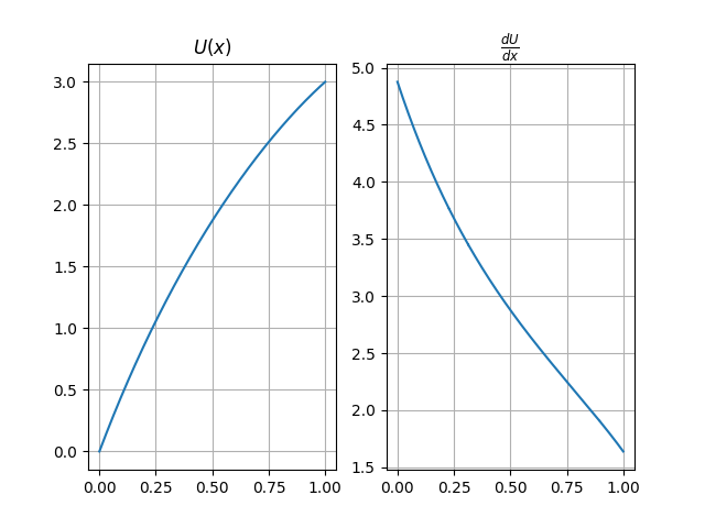
- 1D 1 Variable ordinary diferential equation
- 1D 1 Variable 1D Heat with convective border
- 1D 2 Variable Euler Bernoulli Beams
- 1D 3 Variable Non-linear Euler Bernoulli Beams
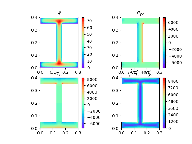
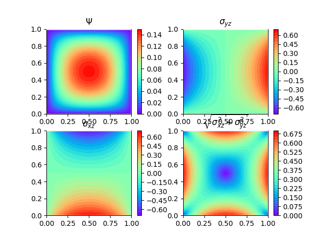
- 2D 1 Variable Torsion
- 2D 1 Variable Poisson equation
- 2D 1 Variable second order PDE
- 2D 1 Variable 2D Heat with convective borders
- 2D 2 Variable Plane Strees
- 2D 2 Variable Plane Strees Orthotropic
- 2D 2 Variable Plane Strain
- 3D 3 variables per node isotropic elasticity
Numerical Validation:
- 1D 1 Variable ordinary diferential equation
- 1D 1 Variable 1D Heat with convective border
- 1D 2 Variable Euler Bernoulli Beams
- 1D 3 Variable Non-linear Euler Bernoulli Beams
- 2D 1 Variable Torsion
- 2D 1 Variable 2D Heat with convective borders
- 2D 2 Variable Plane Strees
- 2D 2 Variable Plane Strain
Steps:
- Create geometry
- Create Border Conditions (Point and regions supported)
- Solve!
- For example: Example 2, Example 5, Example 11-14
Example without geometry file (Test 2):
import matplotlib.pyplot as plt #Import libraries
from FEM.Torsion2D import Torsion2D #import AFEM Torsion class
from FEM.Geometry import Delaunay #Import Meshing tools

#Define some variables with geometric properties
a = 0.3
b = 0.3
tw = 0.05
tf = 0.05

#Define material constants
E = 200000
v = 0.27
G = E / (2 * (1 + v))
phi = 1 #Rotation angle

#Define domain coordinates
vertices = [
        [0, 0],
        [a, 0],
        [a, tf],
        [a / 2 + tw / 2, tf],
        [a / 2 + tw / 2, tf + b],
        [a, tf + b],
        [a, 2 * tf + b],
        [0, 2 * tf + b],
        [0, tf + b],
        [a / 2 - tw / 2, tf + b],
        [a / 2 - tw / 2, tf],
        [0, tf],
]

#Define triangulation parameters with `_strdelaunay` method.
params = Delaunay._strdelaunay(constrained=True, delaunay=True,
                                                                        a='0.00003', o=2)
#**Create** geometry using triangulation parameters. Geometry can be imported from .msh files.
geometry = Delaunay(vertices, params)

#Save geometry to .json file
geometry.exportJSON('I_test.json')

#Create torsional 2D analysis.
O = Torsion2D(geometry, G, phi)
#Solve the equation in domain.
#Post process and show results
O.solve()
plt.show()
Example with geometry file (Example 2):
import matplotlib.pyplot as plt #Import libraries
from FEM.Torsion2D import Torsion2D #import AFEM
from FEM.Geometry import Geometry #Import Geometry tools

#Define material constants.
E = 200000
v = 0.27
G = E / (2 * (1 + v))
phi = 1 #Rotation angle

#Load geometry with file.
geometry = Geometry.importJSON('I_test.json')

#Create torsional 2D analysis.
O = Torsion2D(geometry, G, phi)
#Solve the equation in domain.
#Post process and show results
O.solve()
plt.show()
Creating equation classes
Note: Don't forget the docstring!
Steps
-
Create a Python flie and import the libraries:
from .Core import *
from tqdm import tqdm
import numpy as np
import matplotlib.pyplot as plt
- Core: Solver
- Numpy: Numpy data
- Matplotlib: Matplotlib graphs
- Tqdm: Progressbars
-
Create a Python class with Core inheritance
class PlaneStress(Core):
    def __init__(self,geometry,*args,**kargs):
    #Do stuff
    Core.__init__(self,geometry)
It is important to manage the number of variables per node in the input geometry.
-
Define the matrix calculation methods and post porcessing methods.
def elementMatrices(self):
def postProcess(self):
-
The
elementMatricesmethod uses gauss integration points, so you must use the following structure:for e in tqdm(self.elements,unit='Element'): _x,_p = e.T(e.Z.T) #Gauss points in global coordinates and Shape functions evaluated in gauss points jac,dpz = e.J(e.Z.T) #Jacobian evaluated in gauss points and shape functions derivatives in natural coordinates detjac = np.linalg.det(jac) _j = np.linalg.inv(jac) #Jacobian inverse dpx = _j @ dpz #Shape function derivatives in global coordinates for k in range(len(e.Z)): #Iterate over gauss points on domain #Calculate matrices with any finite element model #Assign matrices to element
A good example is the PlaneStress class in the Elasticity2D.py file.
Roadmap
- 2D elastic plate theory
- Transient analysis (Core modification)
- Non-Lineal for 2D equation (All cases)
- Testing and numerical validation (WIP)
Examples
References
J. N. Reddy. Introduction to the Finite Element Method, Third Edition (McGraw-Hill Education: New York, Chicago, San Francisco, Athens, London, Madrid, Mexico City, Milan, New Delhi, Singapore, Sydney, Toronto, 2006). https://www.accessengineeringlibrary.com/content/book/9780072466850
Jonathan Richard Shewchuk, (1996) Triangle: Engineering a 2D Quality Mesh Generator and Delaunay Triangulator
Ramirez, F. (2020). ICYA 4414 Modelación con Elementos Finitos [Class handout]. Universidad de Los Andes.
License
The Memory Update
Save memoy with sparse matrix!
Docs now behave like first intended
![]()
![]()
A Python FEM implementation.
N dimensional FEM implementation for M variables per node problems.
Installation
Use the package manager pip to install AFEM.
pip install AFEMContributing
Pull requests are welcome. For major changes, please open an issue first to discuss what you would like to change.
Please make sure to update tests as appropriate.
Full Docs
Tutorial
Using pre implemented equations
Avaliable equations:
- 1D 1 Variable ordinary diferential equation
- 1D 1 Variable 1D Heat with convective border
- 1D 2 Variable Euler Bernoulli Beams
- 1D 3 Variable Non-linear Euler Bernoulli Beams
- 2D 1 Variable Torsion
- 2D 1 Variable Poisson equation
- 2D 1 Variable second order PDE
- 2D 1 Variable 2D Heat with convective borders
- 2D 2 Variable Plane Strees
- 2D 2 Variable Plane Strees Orthotropic
- 2D 2 Variable Plane Strain
- 3D 3 variables per node isotropic elasticity
Numerical Validation:
- 1D 1 Variable ordinary diferential equation
- 1D 1 Variable 1D Heat with convective border
- 1D 2 Variable Euler Bernoulli Beams
- 1D 3 Variable Non-linear Euler Bernoulli Beams
- 2D 1 Variable Torsion
- 2D 1 Variable 2D Heat with convective borders
- 2D 2 Variable Plane Strees
- 2D 2 Variable Plane Strain
Steps:
- Create geometry
- Create Border Conditions (Point and regions supported)
- Solve!
- For example: Example 2, Example 5, Example 11-14
Example without geometry file (Test 2):
import matplotlib.pyplot as plt #Import libraries
from FEM.Torsion2D import Torsion2D #import AFEM Torsion class
from FEM.Geometry import Delaunay #Import Meshing tools

#Define some variables with geometric properties
a = 0.3
b = 0.3
tw = 0.05
tf = 0.05

#Define material constants
E = 200000
v = 0.27
G = E / (2 * (1 + v))
phi = 1 #Rotation angle

#Define domain coordinates
vertices = [
        [0, 0],
        [a, 0],
        [a, tf],
        [a / 2 + tw / 2, tf],
        [a / 2 + tw / 2, tf + b],
        [a, tf + b],
        [a, 2 * tf + b],
        [0, 2 * tf + b],
        [0, tf + b],
        [a / 2 - tw / 2, tf + b],
        [a / 2 - tw / 2, tf],
        [0, tf],
]

#Define triangulation parameters with `_strdelaunay` method.
params = Delaunay._strdelaunay(constrained=True, delaunay=True,
                                                                        a='0.00003', o=2)
#**Create** geometry using triangulation parameters. Geometry can be imported from .msh files.
geometry = Delaunay(vertices, params)

#Save geometry to .json file
geometry.exportJSON('I_test.json')

#Create torsional 2D analysis.
O = Torsion2D(geometry, G, phi)
#Solve the equation in domain.
#Post process and show results
O.solve()
plt.show()
Example with geometry file (Example 2):
import matplotlib.pyplot as plt #Import libraries
from FEM.Torsion2D import Torsion2D #import AFEM
from FEM.Geometry import Geometry #Import Geometry tools

#Define material constants.
E = 200000
v = 0.27
G = E / (2 * (1 + v))
phi = 1 #Rotation angle

#Load geometry with file.
geometry = Geometry.importJSON('I_test.json')

#Create torsional 2D analysis.
O = Torsion2D(geometry, G, phi)
#Solve the equation in domain.
#Post process and show results
O.solve()
plt.show()
Creating equation classes
Note: Don't forget the docstring!
Steps
-
Create a Python flie and import the libraries:
from .Core import *
from tqdm import tqdm
import numpy as np
import matplotlib.pyplot as plt
- Core: Solver
- Numpy: Numpy data
- Matplotlib: Matplotlib graphs
- Tqdm: Progressbars
-
Create a Python class with Core inheritance
class PlaneStress(Core):
    def __init__(self,geometry,*args,**kargs):
    #Do stuff
    Core.__init__(self,geometry)
It is important to manage the number of variables per node in the input geometry.
-
Define the matrix calculation methods and post porcessing methods.
def elementMatrices(self):
def postProcess(self):
-
The
elementMatricesmethod uses gauss integration points, so you must use the following structure:for e in tqdm(self.elements,unit='Element'): _x,_p = e.T(e.Z.T) #Gauss points in global coordinates and Shape functions evaluated in gauss points jac,dpz = e.J(e.Z.T) #Jacobian evaluated in gauss points and shape functions derivatives in natural coordinates detjac = np.linalg.det(jac) _j = np.linalg.inv(jac) #Jacobian inverse dpx = _j @ dpz #Shape function derivatives in global coordinates for k in range(len(e.Z)): #Iterate over gauss points on domain #Calculate matrices with any finite element model #Assign matrices to element
A good example is the PlaneStress class in the Elasticity2D.py file.
Roadmap
- 2D elastic plate theory
- Transient analysis (Core modification)
- Non-Lineal for 2D equation (All cases)
- Testing and numerical validation (WIP)
Examples
References
J. N. Reddy. Introduction to the Finite Element Method, Third Edition (McGraw-Hill Education: New York, Chicago, San Francisco, Athens, London, Madrid, Mexico City, Milan, New Delhi, Singapore, Sydney, Toronto, 2006). https://www.accessengineeringlibrary.com/content/book/9780072466850
Jonathan Richard Shewchuk, (1996) Triangle: Engineering a 2D Quality Mesh Generator and Delaunay Triangulator
Ramirez, F. (2020). ICYA 4414 Modelación con Elementos Finitos [Class handout]. Universidad de Los Andes.
License
The Region and Docs Update
![]()
![]()
A Python FEM implementation.
N dimensional FEM implementation for M variables per node problems.
Installation
Use the package manager pip to install AFEM.
pip install AFEMContributing
Pull requests are welcome. For major changes, please open an issue first to discuss what you would like to change.
Please make sure to update tests as appropriate.
Full Docs
Tutorial
Using pre implemented equations
Avaliable equations:
- 1D 1 Variable ordinary diferential equation
- 1D 1 Variable 1D Heat with convective border
- 1D 2 Variable Euler Bernoulli Beams
- 1D 3 Variable Non-linear Euler Bernoulli Beams
- 2D 1 Variable Torsion
- 2D 1 Variable Poisson equation
- 2D 1 Variable second order PDE
- 2D 1 Variable 2D Heat with convective borders
- 2D 2 Variable Plane Strees
- 2D 2 Variable Plane Strees Orthotropic
- 2D 2 Variable Plane Strain
- 3D 3 variables per node isotropic elasticity
Numerical Validation:
- 1D 1 Variable ordinary diferential equation
- 1D 1 Variable 1D Heat with convective border
- 1D 2 Variable Euler Bernoulli Beams
- 1D 3 Variable Non-linear Euler Bernoulli Beams
- 2D 1 Variable Torsion
- 2D 1 Variable 2D Heat with convective borders
- 2D 2 Variable Plane Strees
- 2D 2 Variable Plane Strain
Steps:
- Create geometry
- Create Border Conditions (Point and regions supported)
- Solve!
- For example: Example 2, Example 5, Example 11-14
Example without geometry file (Test 2):
import matplotlib.pyplot as plt #Import libraries
from FEM.Torsion2D import Torsion2D #import AFEM Torsion class
from FEM.Geometry import Delaunay #Import Meshing tools

#Define some variables with geometric properties
a = 0.3
b = 0.3
tw = 0.05
tf = 0.05

#Define material constants
E = 200000
v = 0.27
G = E / (2 * (1 + v))
phi = 1 #Rotation angle

#Define domain coordinates
vertices = [
        [0, 0],
        [a, 0],
        [a, tf],
        [a / 2 + tw / 2, tf],
        [a / 2 + tw / 2, tf + b],
        [a, tf + b],
        [a, 2 * tf + b],
        [0, 2 * tf + b],
        [0, tf + b],
        [a / 2 - tw / 2, tf + b],
        [a / 2 - tw / 2, tf],
        [0, tf],
]

#Define triangulation parameters with `_strdelaunay` method.
params = Delaunay._strdelaunay(constrained=True, delaunay=True,
                                                                        a='0.00003', o=2)
#**Create** geometry using triangulation parameters. Geometry can be imported from .msh files.
geometry = Delaunay(vertices, params)

#Save geometry to .json file
geometry.exportJSON('I_test.json')

#Create torsional 2D analysis.
O = Torsion2D(geometry, G, phi)
#Solve the equation in domain.
#Post process and show results
O.solve()
plt.show()
Example with geometry file (Example 2):
import matplotlib.pyplot as plt #Import libraries
from FEM.Torsion2D import Torsion2D #import AFEM
from FEM.Geometry import Geometry #Import Geometry tools

#Define material constants.
E = 200000
v = 0.27
G = E / (2 * (1 + v))
phi = 1 #Rotation angle

#Load geometry with file.
geometry = Geometry.importJSON('I_test.json')

#Create torsional 2D analysis.
O = Torsion2D(geometry, G, phi)
#Solve the equation in domain.
#Post process and show results
O.solve()
plt.show()
Creating equation classes
Note: Don't forget the docstring!
Steps
-
Create a Python flie and import the libraries:
from .Core import *
from tqdm import tqdm
import numpy as np
import matplotlib.pyplot as plt
- Core: Solver
- Numpy: Numpy data
- Matplotlib: Matplotlib graphs
- Tqdm: Progressbars
-
Create a Python class with Core inheritance
class PlaneStress(Core):
    def __init__(self,geometry,*args,**kargs):
    #Do stuff
    Core.__init__(self,geometry)
It is important to manage the number of variables per node in the input geometry.
-
Define the matrix calculation methods and post porcessing methods.
def elementMatrices(self):
def postProcess(self):
-
The
elementMatricesmethod uses gauss integration points, so you must use the following structure:for e in tqdm(self.elements,unit='Element'): _x,_p = e.T(e.Z.T) #Gauss points in global coordinates and Shape functions evaluated in gauss points jac,dpz = e.J(e.Z.T) #Jacobian evaluated in gauss points and shape functions derivatives in natural coordinates detjac = np.linalg.det(jac) _j = np.linalg.inv(jac) #Jacobian inverse dpx = _j @ dpz #Shape function derivatives in global coordinates for k in range(len(e.Z)): #Iterate over gauss points on domain #Calculate matrices with any finite element model #Assign matrices to element
A good example is the PlaneStress class in the Elasticity2D.py file.
Roadmap
- 2D elastic plate theory
- Transient analysis (Core modification)
- Non-Lineal for 2D equation (All cases)
- Testing and numerical validation (WIP)
Example index:
-
Example 1: Preliminar geometry test
-
Example 2: 2D Torsion 1 variable per node. H section-Triangular Quadratic.
-
Example 3: 2D Torsion 1 variable per node. Square section-Triangular Quadratic.
-
Example 4: 2D Torsion 1 variable per node. Mesh from internet-Square Lineal.
-
Example 5: 2D Torsion 1 variable per node. Creating and saving mesh-Triangular Quadratic.

-
Example 6: 1D random differential equation 1 variable per node. Linear Quadratic.

-
Example 7: GiD Mesh import test — Serendipity elements

-
Example 8: Plane Stress 2 variable per node. Plate in tension — Serendipity.

-
Example 9: Plane Stress 2 variable per node. Simple Supported Beam — Serendipity.

-
Example 10: Plane Stress 2 variable per node. Cantilever Beam — Triangular Quadratic.

-
Example 11: Plane Stress 2 variable per node. Fixed-Fixed Beam — Serendipity.

-
Example 12: Plane Strain 2 variable per node. Embankment from GiD — Serendipity.

-
Example 13: Plane Strain 2 variable per node. Embankment — Triangular Quadratic.


-
Example 14: Plane Stress 2 variable per node. Cantilever Beam — Serendipity.

-
Example 15: Profile creation tool. Same as Example 14

-
Example 16: Non-Local Plane Stress. [WIP]
-
Example 17: 1D Heat transfer.

-
Example 18: 2D border elements creation.

-
Example 19: Apply loads on regions.
loadOnRegionmethod on Test 11
-
Example 20: Reddy's Example 11.7.1 Ed 3
-
Example 21: Exam...
The Region Update
![]()
![]()
A Python FEM implementation.
N dimensional FEM implementation for M variables per node problems.
Installation
Use the package manager pip to install AFEM.
pip install AFEMContributing
Pull requests are welcome. For major changes, please open an issue first to discuss what you would like to change.
Please make sure to update tests as appropriate.
Full Docs
Tutorial
Using pre implemented equations
Avaliable equations:
- 1D 1 Variable ordinary diferential equation
- 1D 1 Variable 1D Heat with convective border
- 1D 2 Variable Euler Bernoulli Beams
- 1D 3 Variable Non-linear Euler Bernoulli Beams
- 2D 1 Variable Torsion
- 2D 1 Variable Poisson equation
- 2D 1 Variable second order PDE
- 2D 1 Variable 2D Heat with convective borders
- 2D 2 Variable Plane Strees
- 2D 2 Variable Plane Strees Orthotropic
- 2D 2 Variable Plane Strain
- 3D 3 variables per node isotropic elasticity
Numerical Validation:
- 1D 1 Variable ordinary diferential equation
- 1D 1 Variable 1D Heat with convective border
- 1D 2 Variable Euler Bernoulli Beams
- 1D 3 Variable Non-linear Euler Bernoulli Beams
- 2D 1 Variable Torsion
- 2D 1 Variable 2D Heat with convective borders
- 2D 2 Variable Plane Strees
- 2D 2 Variable Plane Strain
Steps:
- Create geometry
- Create Border Conditions (Point and regions supported)
- Solve!
- For example: Example 2, Example 5, Example 11-14
Example without geometry file (Test 2):
import matplotlib.pyplot as plt #Import libraries
from FEM.Torsion2D import Torsion2D #import AFEM Torsion class
from FEM.Geometry import Delaunay #Import Meshing tools

#Define some variables with geometric properties
a = 0.3
b = 0.3
tw = 0.05
tf = 0.05

#Define material constants
E = 200000
v = 0.27
G = E / (2 * (1 + v))
phi = 1 #Rotation angle

#Define domain coordinates
vertices = [
        [0, 0],
        [a, 0],
        [a, tf],
        [a / 2 + tw / 2, tf],
        [a / 2 + tw / 2, tf + b],
        [a, tf + b],
        [a, 2 * tf + b],
        [0, 2 * tf + b],
        [0, tf + b],
        [a / 2 - tw / 2, tf + b],
        [a / 2 - tw / 2, tf],
        [0, tf],
]

#Define triangulation parameters with `_strdelaunay` method.
params = Delaunay._strdelaunay(constrained=True, delaunay=True,
                                                                        a='0.00003', o=2)
#**Create** geometry using triangulation parameters. Geometry can be imported from .msh files.
geometry = Delaunay(vertices, params)

#Save geometry to .json file
geometry.exportJSON('I_test.json')

#Create torsional 2D analysis.
O = Torsion2D(geometry, G, phi)
#Solve the equation in domain.
#Post process and show results
O.solve()
plt.show()
Example with geometry file (Example 2):
import matplotlib.pyplot as plt #Import libraries
from FEM.Torsion2D import Torsion2D #import AFEM
from FEM.Geometry import Geometry #Import Geometry tools

#Define material constants.
E = 200000
v = 0.27
G = E / (2 * (1 + v))
phi = 1 #Rotation angle

#Load geometry with file.
geometry = Geometry.importJSON('I_test.json')

#Create torsional 2D analysis.
O = Torsion2D(geometry, G, phi)
#Solve the equation in domain.
#Post process and show results
O.solve()
plt.show()
Creating equation classes
Note: Don't forget the docstring!
Steps
-
Create a Python flie and import the libraries:
from .Core import *
from tqdm import tqdm
import numpy as np
import matplotlib.pyplot as plt
- Core: Solver
- Numpy: Numpy data
- Matplotlib: Matplotlib graphs
- Tqdm: Progressbars
-
Create a Python class with Core inheritance
class PlaneStress(Core):
    def __init__(self,geometry,*args,**kargs):
    #Do stuff
    Core.__init__(self,geometry)
It is important to manage the number of variables per node in the input geometry.
-
Define the matrix calculation methods and post porcessing methods.
def elementMatrices(self):
def postProcess(self):
-
The
elementMatricesmethod uses gauss integration points, so you must use the following structure:for e in tqdm(self.elements,unit='Element'): _x,_p = e.T(e.Z.T) #Gauss points in global coordinates and Shape functions evaluated in gauss points jac,dpz = e.J(e.Z.T) #Jacobian evaluated in gauss points and shape functions derivatives in natural coordinates detjac = np.linalg.det(jac) _j = np.linalg.inv(jac) #Jacobian inverse dpx = _j @ dpz #Shape function derivatives in global coordinates for k in range(len(e.Z)): #Iterate over gauss points on domain #Calculate matrices with any finite element model #Assign matrices to element
A good example is the PlaneStress class in the Elasticity2D.py file.
Roadmap
- 2D elastic plate theory
- Transient analysis (Core modification)
- Non-Lineal for 2D equation (All cases)
- Testing and numerical validation (WIP)
Example index:
-
Example 1: Preliminar geometry test
-
Example 2: 2D Torsion 1 variable per node. H section-Triangular Quadratic.
-
Example 3: 2D Torsion 1 variable per node. Square section-Triangular Quadratic.
-
Example 4: 2D Torsion 1 variable per node. Mesh from internet-Square Lineal.
-
Example 5: 2D Torsion 1 variable per node. Creating and saving mesh-Triangular Quadratic.
-
Example 6: 1D random differential equation 1 variable per node. Linear Quadratic.
-
Example 7: GiD Mesh import test — Serendipity elements
-
Example 8: Plane Stress 2 variable per node. Plate in tension — Serendipity.
-
Example 9: Plane Stress 2 variable per node. Simple Supported Beam — Serendipity.
-
Example 10: Plane Stress 2 variable per node. Cantilever Beam — Triangular Quadratic.
-
Example 11: Plane Stress 2 variable per node. Fixed-Fixed Beam — Serendipity.
-
Example 12: Plane Strain 2 variable per node. Embankment from GiD — Serendipity.
-
Example 13: Plane Strain 2 variable per node. Embankment — Triangular Quadratic.
-
Example 14: Plane Stress 2 variable per node. Cantilever Beam — Serendipity.
-
Example 15: Profile creation tool. Same as Example 14
-
Example 16: Non-Local Plane Stress. [WIP]
-
Example 17: 1D Heat transfer.
-
Example 18: 2D border elements creation.
-
Example 19: Apply loads on regions.
loadOnRegionmethod on Test 11
-
Example 20: Reddy's Example 11.7.1 Ed 3
-
Example 21: Exam...
The elastic update
![]()
![]()
A Python FEM implementation.
N dimensional FEM implementation for M variables per node problems.
Installation
Use the package manager pip to install AFEM.
pip install AFEMContributing
Pull requests are welcome. For major changes, please open an issue first to discuss what you would like to change.
Please make sure to update tests as appropriate.
Full Docs
Tutorial
Using pre implemented equations
Avaliable equations:
- 1D 1 Variable ordinary diferential equation
- 1D 1 Variable 1D Heat with convective border
- 1D 2 Variable Euler Bernoulli Beams
- 1D 3 Variable Non-linear Euler Bernoulli Beams
- 2D 1 Variable Torsion
- 2D 1 Variable Poisson equation
- 2D 1 Variable second order PDE
- 2D 1 Variable 2D Heat with convective borders
- 2D 2 Variable Plane Strees
- 2D 2 Variable Plane Strees Orthotropic
- 2D 2 Variable Plane Strain
- 3D 3 variables per node isotropic elasticity
Numerical Validation:
- 1D 1 Variable ordinary diferential equation
- 1D 1 Variable 1D Heat with convective border
- 1D 2 Variable Euler Bernoulli Beams
- 1D 3 Variable Non-linear Euler Bernoulli Beams
- 2D 1 Variable Torsion
- 2D 1 Variable 2D Heat with convective borders
- 2D 2 Variable Plane Strees
- 2D 2 Variable Plane Strain
Steps:
- Create geometry (From coordinates or GiD)
- Create Border Conditions (Point and segment supported)
- Solve!
- For example: Example 2, Example 5, Example 11-14
Example without geometry file (Test 2):
import matplotlib.pyplot as plt #Import libraries
from FEM.Torsion2D import Torsion2D #import AFEM Torsion class
from FEM.Mesh.Delaunay import Delaunay #Import Meshing tools

#Define some variables with geometric properties
a = 0.3
b = 0.3
tw = 0.05
tf = 0.05

#Define material constants
E = 200000
v = 0.27
G = E / (2 * (1 + v))
phi = 1 #Rotation angle

#Define domain coordinates
vertices = [
        [0, 0],
        [a, 0],
        [a, tf],
        [a / 2 + tw / 2, tf],
        [a / 2 + tw / 2, tf + b],
        [a, tf + b],
        [a, 2 * tf + b],
        [0, 2 * tf + b],
        [0, tf + b],
        [a / 2 - tw / 2, tf + b],
        [a / 2 - tw / 2, tf],
        [0, tf],
]

#Define triangulation parameters with `_strdelaunay` method.
params = Delaunay._strdelaunay(constrained=True, delaunay=True,
                                                                        a='0.00003', o=2)
#**Create** geometry using triangulation parameters. Geometry can be imported from .msh files.
geometry = Delaunay(vertices, params)

#Save geometry to .msh file
geometry.saveMesh('I_test')

#Create torsional 2D analysis.
O = Torsion2D(geometry, G, phi)
#Solve the equation in domain.
#Post process and show results
O.solve()
plt.show()
Example with geometry file (Example 2):
import matplotlib.pyplot as plt #Import libraries
from FEM.Torsion2D import Torsion2D #import AFEM
from FEM.Mesh.Geometry import Geometry #Import Geometry tools

#Define material constants.
E = 200000
v = 0.27
G = E / (2 * (1 + v))
phi = 1 #Rotation angle

#Load geometry with file.
geometry = Geometry.loadmsh('I_test.msh')

#Create torsional 2D analysis.
O = Torsion2D(geometry, G, phi)
#Solve the equation in domain.
#Post process and show results
O.solve()
plt.show()
Creating equation classes
Note: Don't forget the docstring!
Steps
-
Create a Python flie and import the libraries:
from .Core import *
from tqdm import tqdm
import numpy as np
import matplotlib.pyplot as plt
- Core: Solver
- Numpy: Numpy data
- Matplotlib: Matplotlib graphs
- Tqdm: Progressbars
-
Create a Python class with Core inheritance
class PlaneStress(Core):
    def __init__(self,geometry,*args,**kargs):
    #Do stuff
    Core.__init__(self,geometry)
It is important to manage the number of variables per node in the input geometry.
-
Define the matrix calculation methods and post porcessing methods.
def elementMatrices(self):
def postProcess(self):
-
The
elementMatricesmethod uses gauss integration points, so you must use the following structure:for e in tqdm(self.elements,unit='Element'): _x,_p = e.T(e.Z.T) #Gauss points in global coordinates and Shape functions evaluated in gauss points jac,dpz = e.J(e.Z.T) #Jacobian evaluated in gauss points and shape functions derivatives in natural coordinates detjac = np.linalg.det(jac) _j = np.linalg.inv(jac) #Jacobian inverse dpx = _j @ dpz #Shape function derivatives in global coordinates for k in range(len(e.Z)): #Iterate over gauss points on domain #Calculate matrices with any finite element model #Assign matrices to element
A good example is the PlaneStress class in the Elasticity2D.py file.
Roadmap
- 2D elastic plate theory
- Geometry class modification for hierarchy with 1D, 2D and 3D geometry child classes
- Transient analysis (Core modification)
- Non-Lineal for 2D equation (All cases)
- Testing and numerical validation (WIP)
Example index:
-
Example 1: Preliminar geometry test
-
Example 2: 2D Torsion 1 variable per node. H section-Triangular Quadratic.
-
Example 3: 2D Torsion 1 variable per node. Square section-Triangular Quadratic.
-
Example 4: 2D Torsion 1 variable per node. Mesh from internet-Square Lineal.
-
Example 5: 2D Torsion 1 variable per node. Creating and saving mesh-Triangular Quadratic.
-
Example 6: 1D random differential equation 1 variable per node. Linear Quadratic.
-
Example 7: GiD Mesh import test — Serendipity elements
-
Example 8: Plane Stress 2 variable per node. Plate in tension — Serendipity.
-
Example 9: Plane Stress 2 variable per node. Simple Supported Beam — Serendipity.
-
Example 10: Plane Stress 2 variable per node. Cantilever Beam — Triangular Quadratic.
-
Example 11: Plane Stress 2 variable per node. Fixed-Fixed Beam — Serendipity.
-
Example 12: Plane Strain 2 variable per node. Embankment from GiD — Serendipity.
-
Example 13: Plane Strain 2 variable per node. Embankment — Triangular Quadratic.
-
Example 14: Plane Stress 2 variable per node. Cantilever Beam — Serendipity.
-
Example 15: Profile creation tool. Same as Example 14
-
Example 16: Non-Local Plane Stress. [WIP]
-
Example 17: 1D Heat transfer.
-
Example 18: 2D border elements creation.
-
Example 19: Apply loads on segments.
loadOnSegmentmethod on Test 11<img src="https://raw.githubusercontent.com/ZibraMax/FEM/mas...
The Quality of Life Update
![]()
![]()
A Python FEM implementation.
N dimensional FEM implementation for M variables per node problems.
Installation
Use the package manager pip to install AFEM.
pip install AFEMContributing
Pull requests are welcome. For major changes, please open an issue first to discuss what you would like to change.
Please make sure to update tests as appropriate.
Full Docs
Tutorial
Using pre implemented equations
Avaliable equations:
- 1D 1 Variable ordinary diferential equation
- 1D 1 Variable 1D Heat with convective border
- 1D 2 Variable Euler Bernoulli Beams
- 1D 3 Variable Non-linear Euler Bernoulli Beams
- 1D 2 Variable Timoshenko Beams [WIP]
- 2D 1 Variable Torsion
- 2D 1 Variable Poisson equation
- 2D 1 Variable second order PDE
- 2D 1 Variable 2D Heat with convective borders
- 2D 2 Variable Plane Strees
- 2D 2 Variable Plane Strees Orthotropic
- 2D 2 Variable Plane Strain
Numerical Validation:
- 1D 1 Variable ordinary diferential equation
- 1D 1 Variable 1D Heat with convective border
- 1D 2 Variable Euler Bernoulli Beams
- 1D 3 Variable Non-linear Euler Bernoulli Beams
- 1D 2 Variable Timoshenko Beams [WIP]
- 2D 1 Variable Torsion
- 2D 1 Variable 2D Heat with convective borders
- 2D 2 Variable Plane Strees
- 2D 2 Variable Plane Strain
Steps:
- Create geometry (From coordinates or GiD)
- Create Border Conditions (Point and segment supported)
- Solve!
- For example: Example 2, Example 5, Example 11-14
Example without geometry file (Test 2):
import matplotlib.pyplot as plt #Import libraries
from FEM.Torsion2D import Torsion2D #import AFEM Torsion class
from FEM.Mesh.Delaunay import Delaunay #Import Meshing tools

#Define some variables with geometric properties
a = 0.3
b = 0.3
tw = 0.05
tf = 0.05

#Define material constants
E = 200000
v = 0.27
G = E / (2 * (1 + v))
phi = 1 #Rotation angle

#Define domain coordinates
vertices = [
        [0, 0],
        [a, 0],
        [a, tf],
        [a / 2 + tw / 2, tf],
        [a / 2 + tw / 2, tf + b],
        [a, tf + b],
        [a, 2 * tf + b],
        [0, 2 * tf + b],
        [0, tf + b],
        [a / 2 - tw / 2, tf + b],
        [a / 2 - tw / 2, tf],
        [0, tf],
]

#Define triangulation parameters with `_strdelaunay` method.
params = Delaunay._strdelaunay(constrained=True, delaunay=True,
                                                                        a='0.00003', o=2)
#**Create** geometry using triangulation parameters. Geometry can be imported from .msh files.
geometry = Delaunay(vertices, params)

#Save geometry to .msh file
geometry.saveMesh('I_test')

#Create torsional 2D analysis.
O = Torsion2D(geometry, G, phi)
#Solve the equation in domain.
#Post process and show results
O.solve()
plt.show()
Example with geometry file (Example 2):
import matplotlib.pyplot as plt #Import libraries
from FEM.Torsion2D import Torsion2D #import AFEM
from FEM.Mesh.Geometry import Geometry #Import Geometry tools

#Define material constants.
E = 200000
v = 0.27
G = E / (2 * (1 + v))
phi = 1 #Rotation angle

#Load geometry with file.
geometry = Geometry.loadmsh('I_test.msh')

#Create torsional 2D analysis.
O = Torsion2D(geometry, G, phi)
#Solve the equation in domain.
#Post process and show results
O.solve()
plt.show()
Creating equation classes
Note: Don't forget the docstring!
Steps
-
Create a Python flie and import the libraries:
from .Core import *
from tqdm import tqdm
import numpy as np
import matplotlib.pyplot as plt
- Core: Solver
- Core: Numpy data
- Core: Matplotlib graphs
- Tqdm: Progressbars
-
Create a Python class with Core inheritance
class PlaneStress(Core):
    def __init__(self,geometry,*args,**kargs):
    #Do stuff
    Core.__init__(self,geometry)
It is important to manage the number of variables per node in the input geometry.
-
Define the matrix calculation methods and post porcessing methods.
def elementMatrices(self):
def postProcess(self):
-
The
elementMatricesmethod uses gauss integration points, so you must use the following structure:for e in tqdm(self.elements,unit='Element'): _x,_p = e.T(e.Z.T) #Gauss points in global coordinates and Shape functions evaluated in gauss points jac,dpz = e.J(e.Z.T) #Jacobian evaluated in gauss points and shape functions derivatives in natural coordinates detjac = np.linalg.det(jac) _j = np.linalg.inv(jac) #Jacobian inverse dpx = _j @ dpz #Shape function derivatives in global coordinates for k in range(len(e.Z)): #Iterate over gauss points on domain #Calculate matrices with any finite element model #Assign matrices to element
A good example is the PlaneStress class
Roadmap
- Beam bending by Euler Bernoulli and Timoshenko equations
- 2D elastic plate theory
- Geometry class modification for hierarchy with 1D, 2D and 3D geometry child classes
- Transient analysis (Core modification)
- Elasticity in 3D (3D meshing and post process)
- Non-Lineal analysis for 1D equation (All cases)
- Non-Lineal for 2D equation (All cases)
- Testing and numerical validation (WIP)
Example index:
-
Example 1: Preliminar geometry test
-
Example 2: 2D Torsion 1 variable per node. H section-Triangular Quadratic.
-
Example 3: 2D Torsion 1 variable per node. Square section-Triangular Quadratic.
-
Example 4: 2D Torsion 1 variable per node. Mesh from internet-Square Lineal.
-
Example 5: 2D Torsion 1 variable per node. Creating and saving mesh-Triangular Quadratic.
-
Example 6: 1D random differential equation 1 variable per node. Linear Quadratic.
-
Example 7: GiD Mesh import test — Serendipity elements
-
Example 8: Plane Stress 2 variable per node. Plate in tension — Serendipity.
-
Example 9: Plane Stress 2 variable per node. Simple Supported Beam — Serendipity.
-
Example 10: Plane Stress 2 variable per node. Cantilever Beam — Triangular Quadratic.
-
Example 11: Plane Stress 2 variable per node. Fixed-Fixed Beam — Serendipity.
-
Example 12: Plane Strain 2 variable per node. Embankment from GiD — Serendipity.
-
Example 13: Plane Strain 2 variable per node. Embankment — Triangular Quadratic.
-
Example 14: Plane Stress 2 variable per node. Cantilever Beam — Serendipity.
-
Example 15: Profile creation tool. Same as Example 14
-
Example 16: Non-Local Plane Stress. [WIP]
-
Example 17: 1D Heat transfer.
-
Example 18: 2D border elements creation.
<img src="https://raw.githubusercontent.com/ZibraMax/FEM/mas...
The Torsion Update
![]()
![]()
A Python FEM implementation.
N dimensional FEM implementation for M variables per node problems.
Installation
Use the package manager pip to install AFEM.
pip install AFEMContributing
Pull requests are welcome. For major changes, please open an issue first to discuss what you would like to change.
Please make sure to update tests as appropriate.
Full Docs
Tutorial
Using pre implemented equations
Avaliable equations:
- 1D 1 Variable ordinary diferential equation
- 1D 1 Variable 1D Heat with convective border
- 1D 2 Variable Euler Bernoulli Beams [TODO]
- 1D 2 Variable Timoshenko Beams [TODO]
- 2D 1 Variable Torsion
- 2D 1 Variable 2D Heat with convective borders
- 2D 2 Variable Plane Strees
- 2D 2 Variable Plane Strain
Numerical Validation:
- 1D 1 Variable ordinary diferential equation
- 1D 1 Variable 1D Heat with convective border
- 1D 2 Variable Euler Bernoulli Beams [TODO]
- 1D 2 Variable Timoshenko Beams [TODO]
- 2D 1 Variable Torsion
- 2D 1 Variable 2D Heat with convective borders
- 2D 2 Variable Plane Strees
- 2D 2 Variable Plane Strain
Steps:
- Create geometry (From coordinates or GiD)
- Create Border Conditions (Point and segment supported)
- Solve!
- For example: Example 2, Example 5, Example 11-14
Example without geometry file (Test 2):
import matplotlib.pyplot as plt #Import libraries
from FEM.Torsion2D import Torsion2D #import AFEM Torsion class
from FEM.Mesh.Delaunay import Delaunay #Import Meshing tools

#Define some variables with geometric properties
a = 0.3
b = 0.3
tw = 0.05
tf = 0.05

#Define material constants
E = 200000
v = 0.27
G = E / (2 * (1 + v))
phi = 1 #Rotation angle

#Define domain coordinates
vertices = [
        [0, 0],
        [a, 0],
        [a, tf],
        [a / 2 + tw / 2, tf],
        [a / 2 + tw / 2, tf + b],
        [a, tf + b],
        [a, 2 * tf + b],
        [0, 2 * tf + b],
        [0, tf + b],
        [a / 2 - tw / 2, tf + b],
        [a / 2 - tw / 2, tf],
        [0, tf],
]

#Define triangulation parameters with `_strdelaunay` method.
params = Delaunay._strdelaunay(constrained=True, delaunay=True,
                                                                        a='0.00003', o=2)
#**Create** geometry using triangulation parameters. Geometry can be imported from .msh files.
geometry = Delaunay(vertices, params)

#Save geometry to .msh file
geometry.saveMesh('I_test')

#Create torsional 2D analysis.
O = Torsion2D(geometry, G, phi)
#Solve the equation in domain.
#Post process and show results
O.solve()
plt.show()
Example with geometry file (Example 2):
import matplotlib.pyplot as plt #Import libraries
from FEM.Torsion2D import Torsion2D #import AFEM
from FEM.Mesh.Geometry import Geometry #Import Geometry tools

#Define material constants.
E = 200000
v = 0.27
G = E / (2 * (1 + v))
phi = 1 #Rotation angle

#Load geometry with file.
geometry = Geometry.loadmsh('I_test.msh')

#Create torsional 2D analysis.
O = Torsion2D(geometry, G, phi)
#Solve the equation in domain.
#Post process and show results
O.solve()
plt.show()
Creating equation classes
Note: Don't forget the docstring!
Steps
-
Create a Python flie and import the libraries:
from .Core import *
from tqdm import tqdm
import numpy as np
import matplotlib.pyplot as plt
- Core: Solver
- Core: Numpy data
- Core: Matplotlib graphs
- Tqdm: Progressbars
-
Create a Python class with Core inheritance
class PlaneStress(Core):
    def __init__(self,geometry,*args,**kargs):
    #Do stuff
    Core.__init__(self,geometry)
It is important to manage the number of variables per node in the input geometry.
-
Define the matrix calculation methods and post porcessing methods.
def elementMatrices(self):
def postProcess(self):
-
The
elementMatricesmethod uses gauss integration points, so you must use the following structure:for e in tqdm(self.elements,unit='Element'): _x,_p = e.T(e.Z.T) #Gauss points in global coordinates and Shape functions evaluated in gauss points jac,dpz = e.J(e.Z.T) #Jacobian evaluated in gauss points and shape functions derivatives in natural coordinates detjac = np.linalg.det(jac) _j = np.linalg.inv(jac) #Jacobian inverse dpx = _j @ dpz #Shape function derivatives in global coordinates for k in range(len(e.Z)): #Iterate over gauss points on domain #Calculate matrices with any finite element model #Assign matrices to element
A good example is the PlaneStress class
Roadmap
- Beam bending by Euler Bernoulli and Timoshenko equations
- 2D elastic plate theory
- Geometry class modification for hierarchy with 1D, 2D and 3D geometry child classes
- Transient analysis (Core modification)
- Elasticity in 3D (3D meshing and post process)
- Non-Lineal analysis for 1D equation (All cases)
- Non-Lineal for 2D equation (All cases)
- Testing and numerical validation (WIP)
Example index:
-
Example 1: Preliminar geometry test
-
Example 2: 2D Torsion 1 variable per node. H section-Triangular Quadratic.
-
Example 3: 2D Torsion 1 variable per node. Square section-Triangular Quadratic.
-
Example 4: 2D Torsion 1 variable per node. Mesh from internet-Square Lineal.
-
Example 5: 2D Torsion 1 variable per node. Creating and saving mesh-Triangular Quadratic.
-
Example 6: 1D random differential equation 1 variable per node. Linear Quadratic.
-
Example 7: GiD Mesh import test — Serendipity elements
-
Example 8: Plane Stress 2 variable per node. Plate in tension — Serendipity.
-
Example 9: Plane Stress 2 variable per node. Simple Supported Beam — Serendipity.
-
Example 10: Plane Stress 2 variable per node. Cantilever Beam — Triangular Quadratic.
-
Example 11: Plane Stress 2 variable per node. Fixed-Fixed Beam — Serendipity.
-
Example 12: Plane Strain 2 variable per node. Embankment from GiD — Serendipity.
-
Example 13: Plane Strain 2 variable per node. Embankment — Triangular Quadratic.
-
Example 14: Plane Stress 2 variable per node. Cantilever Beam — Serendipity.
-
Example 15: Profile creation tool. Same as Example 14
-
Example 16: Non-Local Plane Stress. [WIP]
-
Example 17: 1D Heat transfer.
-
Example 18: 2D border elements creation.
-
Example 19: Apply loads on segments.
loadOnSegmentmethod on Test 11<img src="https://raw.githubusercontent.com/ZibraMax/FEM/master/Examples/ex...