> git clone https://github.com/abyzovlab/CNVpytor.git
> cd CNVpytor
> python setup.py install
For single user (without admin privileges) use:
> python setup.py install --user
Old version (v1.0) is available using pip directly (not recommended at the moment):
> pip install cnvpytor
> cnvpytor -download
Second line will download resource files from GitHub.
Make sure that you have indexed alignment (SAM, BAM or CRAM) file.
Initialize your CNVpytor project by running:
> cnvpytor -root file.pytor -rd file.bam [-chrom name1 ...] [-T ref.fa.gz]
where:
- file.pytor -- specifies output cnvpytor file (HDF5 file)
- name1 ... -- specifies chromosome name(s).
- file.bam -- specifies bam/sam/cram file name.
- -T ref.fa.gz -- specifies reference genome file (only for cram file without reference genome).
Chromosome names must be specified the same way as they are described in the sam/bam/cram header, e.g., chrX or X. One can specify multiple chromosomes separated by space. If no chromosome is specified, read mapping is extracted for all chromosomes in the sam/bam file. Note that the pytor file is not being overwritten.
Examples:
> cnvpytor -root NA12878.pytor -chrom 1 2 3 -rd NA12878_ali.bam
for bam files with a header like this:
@HD VN:1.4 GO:none SO:coordinate
@SQ SN:1 LN:249250621
@SQ SN:2 LN:243199373
@SQ SN:3 LN:198022430
or
> cnvpytor -root NA12878.pytor -chrom chr1 chr2 chr3 -rd NA12878_ali.bam
for bam files with a header like this:
@HD VN:1.4 GO:none SO:coordinate
@SQ SN:chr1 LN:249250621
@SQ SN:chr2 LN:243199373
@SQ SN:chr3 LN:198022430
After -rd step file file.pytor is created and read depth data binned to 100 base pair bins will be stored in pytor file.
Chromosome names and lengths are parsed from the input file header and used to detect reference genome.
Reference genome is important for GC correction and 1000 genome strict mask filtering. CNVpytor installation includes human genomes hg19 and hg38 with data files that provide information about GC content and strict mask. For other species or reference genomes you have to configure reference genome (see example).
To check is reference genome detected use:
> cnvpytor -root file.pytor -ls
CNVpytor will print out details about file.pytor including line that specify which reference genome is used and are there available GC and mask data:
Using reference genome: hg19 [ GC: yes, mask: yes ]
Command -ls is useful if you want to check content of pytor file but also date and version of cnvpytor that created it.
First we have to chose bin size. By cnvpytor design it have to be divisible by 100. Here we will use 10 kbp and 100 kbp bins.
To calculate read depth histograms, GC correction and statistics type:
> cnvpytor -root file.pytor -his 10000 100000
Next step is partitioning using mean-shift method:
> cnvpytor -root file.pytor -partition 10000 100000
Finally we can call CNV regions using commands:
> cnvpytor -root file.pytor -call 10000 > calls.10000.tsv
> cnvpytor -root file.pytor -call 100000 > calls.100000.tsv
Result is stored in tab separated files with following columns:
- CNV type: "deletion" or "duplication",
- CNV region (chr:start-end),
- CNV size,
- CNV level - read depth normalized to 1,
- e-val1 -- e-value (p-value multiplied by genome size divided by bin size) calculated using t-test statistics between RD statistics in the region and global,
- e-val2 -- e-value (p-value multiplied by genome size divided by bin size) from the probability of RD values within the region to be in the tails of a gaussian distribution of binned RD,
- e-val3 -- same as e-val1 but for the middle of CNV,
- e-val4 -- same as e-val2 but for the middle of CNV,
- q0 -- fraction of reads mapped with q0 quality in call region,
- pN -- fraction of reference genome gaps (Ns) in call region,
- dG -- distance from closest large (>100bp) gap in reference genome.
Using viewer mode we can filter calls based on five parameters: CNV size, e-val1, q0, pN and dG:
> cnvpytor -root file.pytor [file2.pytor ...] -view 10000

cnvpytor> set Q0_range -1 0.5        # filter calls with more than half not uniquely mapped reads
cnvpytor> set p_range 0 0.0001       # filter non-confident calls
cnvpytor> set p_N 0 0.5              # filter calls with more than 50% Ns in reference genome
cnvpytor> set size_range 50000 inf   # filter calls smaller than 50kbp
cnvpytor> set dG_range 100000 inf    # filter calls close to gaps in reference genome (<100kbp)
cnvpytor> print calls                # printing calls on screen (tsv format)
...
...
cnvpytor> set print_filename file.xlsx   # output filename (xlsx, tsv or vcf)
cnvpytor> set annotate               # turn on annotation (optional - takes a lot of time)
cnvpytor> print calls                # generate output file with filtered calls
cnvpytor> quit
Upper bound for parameters size_range and dG_range can be inf (infinity).
If there are multiple samples (pytor files) there will be an additional column with sample name in tsv format, multiple sheets in Excel format, and multiple sample columns in vcf format.
To import variant data from VCF file use following command:
> cnvpytor -root file.pytor -snp file.vcf.gz [-sample sample_name] [-chrom name1 ...] [-ad AD_TAG] [-gt GT_TAG] [-noAD]
where:
- file.pytor -- specifies cnvpytor file,
- file.vcf -- specifies variant file name.
- sample_name -- specifies VCF sample name,
- name1 ... -- specifies chromosome name(s),
- -ad AD_TAG -- specifies AD tag used in vcf file (default AD)
- -gt GT_TAG -- specifies GT tag used in vcf file (default GT)
- -noAD -- ref and alt read counts will not be readed (see next section)
Chromosome names must be specified the same way as they are described in the vcf header, e.g., chrX or X. One can specify multiple chromosomes separated by space. If no chromosome is specified, all chromosomes from the vcf file will be parsed.
If chromosome names in variant and alignment file are different in prefix chr (e.g. in "1" and "chr1") cnvpytor will detect it and match the names using first imported name for both signals.
In some cases it is useful to read positions of SNPs from vcf file and extract read counts from bam file. For example if we have two samples, normal tissue and cancer, normal can be used to call germline SNPs, while samtools mpileup procedure can be used to calculate read counts in cancer sample at the positions of SNPs. CNVpytor have implemented this procedure. After reading SNP positions (previous step) type:
> cnvpytor -root file.pytor -pileup file.bam [-T ref.fa.gz]
where
- file.pytor -- specifies cnvpytor file,
- file.bam -- specifies bam/sam/cram file,
- -T ref.fa.gz -- specifies reference genome file (only for cram file without reference genome).
To apply 1000 genomes strict mask filter:
> cnvpytor -root file.pytor -mask_snps
To calculate baf histograms for maf, baf and likelihood function for baf use:
> cnvpytor -root file.pytor -baf 10000 100000 [-nomask]
Finally we can call CNV regions using commands:
> cnvpytor -root file.pytor -call combined 10000 > calls.combined.10000.tsv
> cnvpytor -root file.pytor -call combined 100000 > calls.combined.100000.tsv
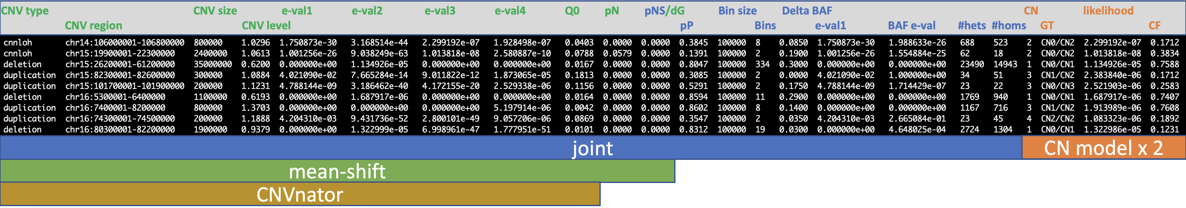
Result is stored in tab separated files with following columns:
- CNV type: "deletion", "duplication", or ”cnnloh",
- CNV region (chr:start-end),
- CNV size,
- CNV level - read depth normalized to 1,
- e-val1 -- e-value (p-value multiplied by genome size divided by bin size) calculated using t-test statistics between RD statistics in the region and global,
- e-val2 -- e-value (p-value multiplied by genome size divided by bin size) from the probability of RD values within the region to be in the tails of a gaussian distribution of binned RD,
- e-val3 -- same as e-val1 but for the middle of CNV,
- e-val4 -- same as e-val2 but for the middle of CNV,
- q0 -- fraction of reads mapped with q0 quality in call segments,
- pN -- fraction of reference genome gaps (Ns) within call region,
- pNS -- fraction of reference genome gaps (Ns) within call segments,
- pP -- fraction of P bases (1kGP strict mask) within call segments,
- bin_size – size of bins
- n – number of bins within call segments,
- delta_BAF – change in BAF from ½,
- e-val1 -- e-value RD based (repeted, reserved for future upgrades),
- baf_eval – e-value BAF based,
- hets – number of HETs,
- homs – number of HOMs,
- cn_1 – most likely model copy number,
- genotype_1 - most likely model genotype,
- likelihood_1 – most likely model likelihood,
- cf_1 -- most likely model cell fraction,
- cn_2 – the second most likely model copy number,
- genotype_2 - the second most likely model genotype,
- likelihood_2 – the second most likely model likelihood,
- cf_2 -- the second most likely model cell fraction.
Using viewer mode we can filter calls based on five parameters: CNV size, e-val1, q0, pN and dG:
> cnvpytor -root file.pytor [file2.pytor ...] -view 10000
cnvpytor> set caller combined_mosaic # IMPORTANT, default caller is mean shift
cnvpytor> set Q0_range -1 0.5        # filter calls with more than half not uniquely mapped reads
cnvpytor> set p_range 0 0.0001       # filter non-confident calls
cnvpytor> set p_N 0 0.5              # filter calls with more than 50% Ns in reference genome
cnvpytor> set size_range 50000 inf   # filter calls smaller than 50kbp
cnvpytor> set dG_range 100000 inf    # filter calls close to gaps in reference genome (<100kbp)
cnvpytor> print calls                # printing calls on screen (tsv format)
...
...
cnvpytor> set print_filename file.xlsx   # output filename (xlsx, tsv or vcf)
cnvpytor> set annotate               # turn on annotation (optional - takes a lot of time)
cnvpytor> print calls                # generate output file with filtered calls
cnvpytor> quit
Upper bound for parameters size_range and dG_range can be inf (infinity).
If there are multiple samples (pytor files) there will be an additional column with sample name in tsv format, multiple sheets in Excel format, and multiple sample columns in vcf format.
Comparison between CNVnator and CNVpytor callers output format:
Using -genotype option followed by bin_sizes you can enter region and genotype calculation for each bin size will be performed:
> cnvpytor -root file.pytor -genotype 10000 100000
12:11396601-11436500
12:11396601-11436500    1.933261    1.937531
22:20999401-21300400
22:20999401-21300400    1.949186    1.957068
Genotyping with additional information:
> cnvpytor -root file.pytor -genotype 10000 -a [-rd_use_mask] [-nomask]
12:11396601-11436500
12:11396601-11436500    2.0152  1.629621e+04    9.670589e+08    0.0000  0.0000  4156900 1.0000  50      4       0.0000  1.000000e+00
Output columns are:
- region,
- cnv level -- mean RD normalized to mean autosomal RD level,
- e_val_1 -- p value calculated using t-test statistics between RD statistics in the region and global,
- e_val_2 -- p value from the probability of RD values within the region to be in the tails of a gaussian distribution of binned RD,
- q0 – fraction of reads mapped with q0 quality within call region,
- pN – fraction of reference genome gaps (Ns) within call region,
- dG -- distance from closest large (>100bp) gap in reference genome,
- proportion of bins used in RD calculation (with option -rd_use_mask some bins can be filtered out),
- Number of homozygous variants within region,
- Number of heterozygous variants,
- BAF level (difference from 0.5) for HETs estimated using maximum likelihood method,
- p-value based on BAF signal.
Option -rd_use_mask turns on P filtering (1000 Genome Project strict mask) for RD signal.
Option -nomak turns off P filtering of SNPs (1000 Genome Project strict mask) for BAF signal.
Example:
Genotype all called CNVs:
> awk '{ print $2 }' calls.10000.tsv | cnvpytor -root file.pytor -genotype 10000 100000
Chromosome wide plots:
> cnvpytor -root file.pytor -plot [rd BIN_SIZE] [likelihood BIN_SIZE] [baf BIN_SIZE] [snp] [-o IMAGE_FILENAME]
where
- rd BIN_SIZE -- plots RD signal for all chromosomes
- likelihood BIN_SIZE -- plots baf likelihood for all chromosomes
- baf BIN_SIZE -- plots baf/maf/likelihood peak position for all chromosomes
- snp -- plots baf for each snp for all chromosomes
- -o IMAGE_FILENAME -- if specified, saves plot in file instead to show on the screen
Manhattan plot:
> cnvpytor -root file.pytor -plot manhattan BIN_SIZE [-chrom name1 ...] [-o IMAGE_FILENAME]
Circular plot:
> cnvpytor -root file.pytor -plot circular BIN_SIZE [-chrom name1 ...] [-o IMAGE_FILENAME]
Plot genomic regions:
> cnvpytor -root file.pytor -plot regions [reg1[,| ]...] BIN_SIZE [-panels [rd] [likelihood] [baf] [snp] ...] [-o IMAGE_FILENAME]
where
- reg1 -- comma or space separated regions in form CHR[:START-STOP], e.g. 1:1M-20M 2 3:200k-80000010
- if regions are comma separated they will be plotted in the same subplot
- space will split regions in different subplots
- -panels -- specify which panels to plot: rd likelihood baf snp
- -o IMAGE_FILENAME -- if specified, saves plot in file instead to show on the screen
The best way to visualize cnvpytor results is interactive mode. Enter interactive mode by typing:
cnvpytor -root file.pytor -view BIN_SIZE
There is tab completion and help similar to man pages. Type double tab or help to start.
Visualize CNVpytor data inside JBrowse
JBrowse version: https://github.com/GMOD/jbrowse/archive/1.16.6-release.tar.gz
Plugins:
- multibigwig (https://github.com/elsiklab/multibigwig )
- multiscalebigwig (https://github.com/cmdcolin/multiscalebigwig)
Note: The JBrowse development version is required as integration of different jbrowse plugins are needed.
To generate cnvpytor file for JBrowse visualization:
cnvpytor -root [pytor files] -export jbrowse [optional argument: output path]

Default export directory name:
 - For single pytor file input:  jbrowse_[pytor file name]
 - For multiple pytor file input: cnvpytor_jbrowse_export
The above command creates all the necessary files that are required to visualize the cnvpytor data.
To view cnvpytor file using JBrowse, users need to install JBrowse and required plugins (See JBrowse version and plugins section).
http://localhost/jbrowse/?data=[export directory]
# Example usage
cnvpytor -root test.pytor -export jbrowse
http://localhost/jbrowse/?data=jbrowse_test
There are mainly two types of data cnvpytor processes. i.e.; Read depth data from alignment file and SNP data from variant file. Depending on the availability of these two input data, the export function works.
For Read depth data, it exports Raw segmented RD, GC corrected Raw Segmented RD, GC corrected RD partition, CNV calling using RD . All of these Read depth signals are plotted on top of each other on a single horizontal track using color gray, black, red and green respectively. For SNP data, it exports Binned BAF, Likelihood of the binned BAF signals. These two signals are plotted on top of each other with gray and red color.
| Data | Signal name with color on JBrowse |
|---|---|
| Read Depth (RD) | Raw Segmented RD (Gray) GC Corrected Raw Segmented RD (Black) GC corrected RD partition (Red) CNV call using RD signals (Green) |
| SNP | Binned BAF (Gray) Likelihood of the Binned BAF (Red) |
cnvpytor does the segmentation for all of the above data based on the user provided bin size. The multiscalebigwig provides the option to show the data based on the visualized area on the reference genome, which means if a user visualizes a small region of the genome it shows small bin data and vice versa.