JavaScript Algorithmic Interview Questions And Considerations

Order the common complexity classes according to their growth rate

Videos

• Abdul Bari: YouTubeChannel for Algorithms
• Data Structures and algorithms
• Data Structures and algorithms Course
• Khan Academy
• Data structures by mycodeschoolPre-requisite for this lesson is good understanding of pointers in C.
• MIT 6.006: Intro to Algorithms(2011)
• Data Structures and Algorithms by Codewithharry

Books

• Introduction to Algorithms by Thomas H. Cormen, Charles E. Leiserson, Ronald L. Rivest, and Clifford Stein
• Competitive Programming 3 by Steven Halim and Felix Halim
• Competitive Programmers Hand Book Beginner friendly hand book for competitive programmers.
• Data Structures and Algorithms Made Easy by Narasimha Karumanchi
• Learning Algorithms Through Programming and Puzzle Solving by Alexander Kulikov and Pavel Pevzner

Coding practice

• LeetCode
• InterviewBit
• Codility
• HackerRank
• Project Euler
• Spoj
• Google Code Jam practice problems
• HackerEarth
• Top Coder
• CodeChef
• Codewars
• CodeSignal
• CodeKata
• Firecode

Courses

• Master the Coding Interview: Big Tech (FAANG) Interviews Course by Andrei and his team.
• Common Python Data Structures Data structures are the fundamental constructs around which you build your programs. Each data structure provides a particular way of organizing data so it can be accessed efficiently, depending on your use case. Python ships with an extensive set of data structures in its standard library.
• Fork CPP A good course for beginners.
• EDU Advanced course.
• C++ For Programmers Learn features and constructs for C++.

Guides

• GeeksForGeeks --- A CS portal for geeks
• Learneroo --- Algorithms
• Top Coder tutorials
• Infoarena training path (RO)
• Steven & Felix Halim --- Increasing the Lower Bound of Programming Contests (UVA Online Judge)

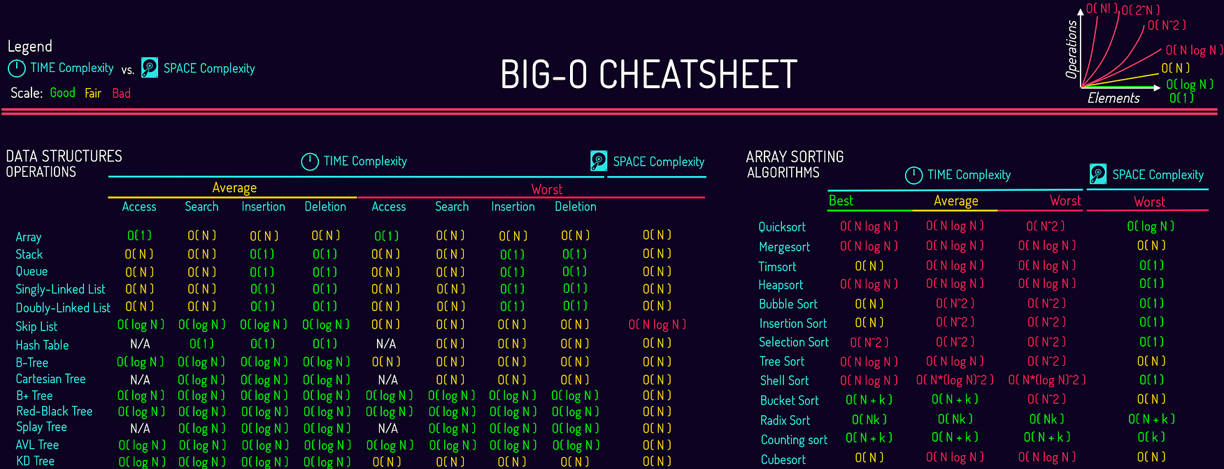
The space complexity represents the memory consumption of a data structure. As for most of the things in life, you can't have it all, so it is with the data structures. You will generally need to trade some time for space or the other way around.

The time complexity for a data structure is in general more diverse than its space complexity.

In contrary to algorithms, when you look at the time complexity for data structures you need to express it for several operations that you can do with data structures. It can be adding elements, deleting elements, accessing an element or even searching for an element.

Something that data structure and algorithms have in common when talking about time complexity is that they are both dealing with data. When you deal with data you become dependent on them and as a result the time complexity is also dependent of the data that you received. To solve this problem we talk about 3 different time complexity.

• The best-case complexity: when the data looks the best
• The worst-case complexity: when the data looks the worst
• The average-case complexity: when the data looks average

The complexity is usually expressed with the Big O notation. The wikipedia page about this subject is pretty complex but you can find here a good summary of the different complexity for the most famous data structures and sorting algorithms.

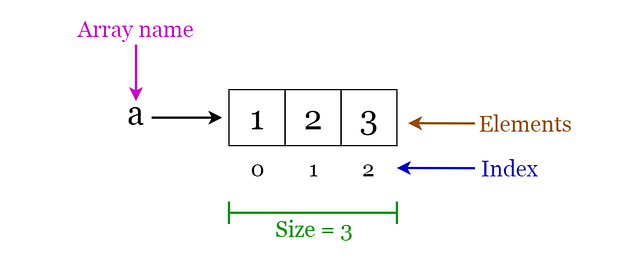
An Array data structure, or simply an Array, is a data structure consisting of a collection of elements (values or variables), each identified by at least one array index or key. The simplest type of data structure is a linear array, also called one-dimensional array. From Wikipedia

Arrays are among the oldest and most important data structures and are used by every program. They are also used to implement many other data structures.

Let's think about how we would implement an array... (a native data structure that will form the basis for most of our abstract data structures)

result:

const array = new ArrayADT(); ArrayADT { array: [] }-------------------------------array.add(1): undefinedarray.add(2); : undefined array.add(3); undefined array.add(4); undefined-------------------------------1 3 4 2 3 4-------------------------------search 3 gives index 2: null-------------------------------getAtIndex 2 gives 3: 4-------------------------------length is 4: 6-------------------------------1 4 2 4-------------------------------1 4 2 4 5 5-------------------------------1 4 2 4-------------------------------const array = new ArrayADT(); : ArrayADT { array: [] }

Big-O

Order the common complexity classes according to their growth rate

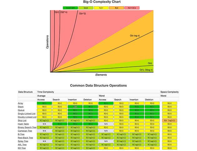
The following are in order from smallest growth (most efficient) to largest:

BEST

constant O(1)

logarithmic O(log n)

linear O(n)

loglinear, linearithmic, quasilinear O(n log n)

polynomial O(n^c) -> O(n²), O(n³)

exponential O(c^n) -> O(2^n), O(3^n)

factorial O(n!)

WORST

Identify the complexity classes of common sort methods

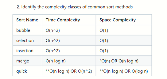
*merge sort can be O(n) space complexity

• if we are not creating a new array every time we call merge sort on the left and right side. We can make it O(n) if we keep track of the start and end index of the left/right sides in the original array and pass that into the merge sort calls to the left and right side. In the way we implement, merge sort's space complexity is O(n log n) because we create a new array to pass into each call of merge sort to the left and right sides.

**quick sort's complexities are a little more complicated

• We are generally only concerned with the worst-scenario when we talk Big-O.
• With quick sort, the worst case is exceedingly rare (only occurs when our pivot for each round happens to be the next element, resulting in us having to choose n pivot points)
• Because it is so rare that this occurs, most people will use consider quick sort to be closer to O(n log n) time complexity.
• We also have two space complexities listed. The version that we used in class creates a new array for every call to quicksort, resulting in O(n log n) space. With some tweaking, we can sort in place, modifying the original array and cutting our space complexity to O(log n), which is just a result of the stack frames that we have to create. It's good to know this method exists, but you will not need to create or identify this version.

Identify complexity classes of code

Memoization and Tabulation

Apply memoization to recursive problems to make them less than polynomial time.

Main steps for memoizing a problem:

1.) Write out the brute force recursion

2.) Add the memo object as an additional argument

Keys on this object represent input, values are the corresponding output

3.) Add a base condition that returns the stored value if the argument is already in the memo

4.) Before returning a calculation, store the result in the memo for future use

Example of a standard and memoized Fibonacci:

Apply tabulation to iterative problems to make them less than polynomial time.

Main considerations for using tabulation:

• Figure out how big is your table
• Typically going to be base on input size (number in Fibonacci, length of string in wordbreak)
• What does my table represent?
• You are generally building up your answer.
• In Fibonacci, we used the table to store the fib number at the corresponding index.
• In stepper, we stored the Boolean of whether it was possible to get to that location.
• What initial values do I need to seed?
• Consider what your end result should be (Boolean, number, etc.).
• Your seed data is generally going to be the immediate answer that we know from our base condition.
• In Fibonacci, we knew the first two numbers of the series.
• In stepper, we knew that it was possible to get to our starting location, so we seeded it as true, defaulting the rest to false so that we could later change its value if we could make that step.
• How do I iterate and fill out my table?
• We typically need to iterate over or up to our input in some way in order to update and build up our table until we get our final result.
• In Fibonacci, we iterated up to our input number in order to calculate the fib number at each step.
• In stepper, we iterated over each possible stepping location. If we could have made it to that point from our previous steps (ie that index was true in our table), we continued updating our table by marking the possible landing spots as true.

Example of a tabulated Fibonacci:

Sorting Algorithms

binary search:

bubble sort:

insertion sort:

merge sort:

quick sort:

selection sort:

Explain the complexity of and write a function that performs bubble sort on an array of numbers.

Time Complexity: O(n²)

• In our worst case, our input is in the opposite order. We have to perform n swaps and loop through our input n times because a swap is made each time.

Space Complexity: O(1)

• We are creating the same number of variables with an exact size, independent of our input. No new arrays are created.

Code example for bubbleSort:

Explain the complexity of and write a function that performs selection sort on an array of numbers.

Time Complexity: O(n²)

• Our nested loop structure is dependent on the size of our input.
• The outer loop always occurs n times.
• For each of those iterations, we have another loop that runs (n --- i) times. This just means that the inner loop runs one less time each iteration, but this averages out to (n/2).
• Our nested structure is then T(n * n/2) = O(n²)

Space Complexity: O(1)

• We are creating the same number of variables with an exact size, independent of our input. No new arrays are created.

Code example for selectionSort:

Explain the complexity of and write a function that performs insertion sort on an array of numbers.

Time Complexity: O(n²)

• Our nested loop structure is dependent on the size of our input.
• The outer loop always occurs n times.
• For each of those iterations, we have another loop that runs a maximum of (i --- 1) times. This just means that the inner loop runs one more time each iteration, but this averages out to (n/2).
• Our nested structure is then T(n * n/2) = O(n²)

Space Complexity: O(1)

• We are creating the same number of variables with an exact size, independent of our input. No new arrays are created.

Code example for insertionSort:

Explain the complexity of and write a function that performs merge sort on an array of numbers.

Time Complexity: O(n log n)

• Our mergeSort function divides our input in half at each step, recursively calling itself with smaller and smaller input. This results in log n stack frames.
• On each stack frame, our worst case scenario is having to make n comparisons in our merge function in order to determine which element should come next in our sorted array.
• Since we have log n stack frames and n operations on each frame, we end up with an O(n log n) time complexity

Space Complexity: O(n log n)

• We are ultimately creating n subarrays for every log n stack frames, making our space complexity quasilinear to our input size.
• IDEALLY merge sort space complexity is O(n) see merge sort space complexity explanation

Code example for mergeSort:

Explain the complexity of and write a function that performs quick sort on an array of numbers.

Time Complexity: Average O(n log n), Worst O(n²)

• In our worst case, the pivot that we select results in every element going into either the left or right array. If this happens we end up making n recursive calls to quickSort, with n comparisons at each call.
• In our average case, we pick something that more evenly splits the arrays, resulting in approximately log n recursive calls and an overall complexity of O(n log n).
• Quick sort is unique in that the worst case is so exceedingly rare that it is often considered an O(n log n) complexity, even though this is not technically accurate.

Space Complexity: Our implementation O(n), Possible implementation O(log n)

• The partition arrays that we create are directly proportional to the size of the input, resulting in O(n) space complexity.
• With some tweaking, we could implement an in-place quick sort, which would eliminate the creation of new arrays. In this case, the log n stack frames from the recursion are the only proportional amount of space that is used, resulting in O(log n) space complexity.

Code example for quickSort:

Explain the complexity of and write a function that performs a binary search on a sorted array of numbers.

Time Complexity: O(log n)

• With each recursive call, we split our input in half. This means we have to make at most log n checks to know if the element is in our array.

Space Complexity: Our implementation O(n), Possible implementation O(1)

• We have to make a subarray for each recursive call. In the worst case (we don't find the element), the total length of these arrays is approximately equal to the length of the original (n).
• If we kept references to the beginning and end index of the portion of the array that we are searching, we could eliminate the need for creating new subarrays. We could also use a while loop to perform this functionality until we either found our target or our beginning and end indices crossed. This would eliminate the space required for recursive calls (adding stack frames). Ultimately we would be using the same number of variables independent of input size, resulting in O(1).

Code example for binarySearch and binarySearchIndex:

Lists, Stacks, and Queues

• Do the projects over and see make sure to know the following

Explain and implement a Linked List.

• A linked list are a collection of ordered data that track three main components:
• head: beginning of the list
• tail: end of the list
• length: count of the number of elements in the list
• The main differences between lists and arrays are that a list does not have random access or indices to signify where in the list an element is.
• The only references to elements that we have in a list are the head and the tail.
• If we want an element in the middle of the list, we would have to traverse the list until we encountered it.
• The two main types of linked lists that we talked about are Singly Linked Lists and Doubly Linked Lists.
• Singly Linked Lists are composed of nodes that only have a reference to the next node in the list. We can only traverse the list in one direction.
• Doubly Linked Lists are composed of nodes that have a reference to both the next node and the previous node in the list. This allows us to traverse both forwards and backwards.

Methods of a linked list that we should know are:

• addToTail: Adds a new node to the end of the list.
• addToHead: Adds a new node to the front of the list.
• insertAt: Adds a new node at the specified position (we need to traverse to that point, then update pointers)
• removeTail: Removes the last node of the list.
• removeHead: Removes the first node of the list.
• removeFrom: Removes the node at the specified position.
• contains: Traverses the list and returns a Boolean to indicate if the value was found at any node.
• get: Returns a reference to the node at the specified position.
• set: Updates the value of the node at the specified position.
• size: Returns the current length of the list.

Time complexities for these methods:

• Accessing a node: O(n), because we may have to traverse the entire list.
• Searching a list: O(n), because we may have to traverse the entire list.
• Inserting a value: O(1), under the assumption that we have a reference to the node that we want to insert it after/before. If we don't have this reference we would first have to access it (O(n) from above), but the actual creation is O(1)
• Deleting a node: O(1), for the same reasons as insertion. If we first need to find the previous and next nodes, we would need to access them (O(n) from above), but the actual deletion is O(1)
• Be able to implement a Singly Linked List and a Doubly Linked List. This would require you to use a Node class with a value instance variable and an instance variable that points to the next (and possibly previous) Node instance(s). You should then be able to interact with these Nodes to perform all of the actions of a Linked List, as we defined above.

Explain and implement a Stack.

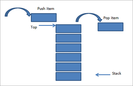
• A Last In First Out (LIFO) Abstract Data Type (ADT).
• LIFO: The last element put into the stack is the first thing removed from it. Think of it as a can of Pringles or a pile of dishes.
• ADT: The actual implementation of the stack can vary as long as the main principles and methods associated with them are abided by. We could use Nodes like we did with Linked Lists, we could use an Array as an underlying instance variable as long as the methods we implement only interact with it in the way a stack should be interacted with, etc.

Methods of a Stack we should know are:

• push: Adds an element to the top of the stack.
• pop: Removes an element from the top of the stack.
• peek: Returns the value of the top element of the stack.
• size: Returns the number of elements in the stack.

Time Complexities:

• Adding an element: O(1), since we are always adding it to the top and the addition doesn't affect any other elements.
• Removing an element: O(1), we're always taking the top element of the stack.
• Finding or Accessing a particular element: O(n), since we can only interact with our stack by removing elements from the top, we may have to remove every element to find what we're looking for.

Explain and implement a Queue.

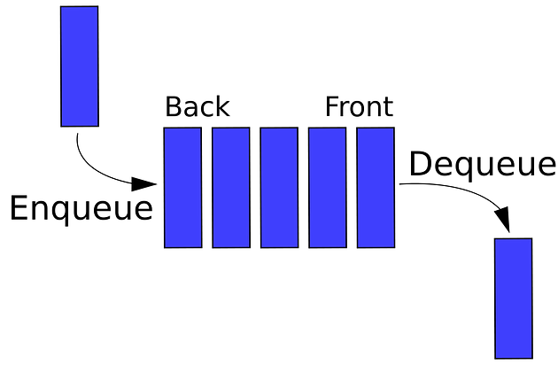
• A First In First Out (FIFO OR LILO) Abstract Data Type (ADT).
• FIFO: The first element put into the queue is the first thing removed from it. Think of it as if you are waiting in line at a store, first come, first serve.
• ADT: The actual implementation of the queue can vary as long as the main principles and methods associated with them are abided by. We could use Nodes like we did with Linked Lists, we could use an Array as an underlying instance variable as long as the methods we implement only interact with it in the way a queue should be interacted with, etc.

Methods of a Queue we should know are:

• enqueue: Adds an element to the back of the queue.
• dequeue: Removes an element from the front of the queue.
• peek: Returns the value of the front element of the queue.
• size: Returns the number of elements in the queue.

Time Complexities:

• Adding an element: O(1), since we are always adding it to the back. If we are using Nodes instead of a simple array, keeping a reference to the last node allows us to immediately update these pointers without having to do any traversal.
• Removing an element: O(1), we're always taking the front element of the queue.
• Finding or Accessing a particular element: O(n), since we can only interact with our queue by removing elements from the front, we may have to remove every element to find what we're looking for.

MY BLOG: