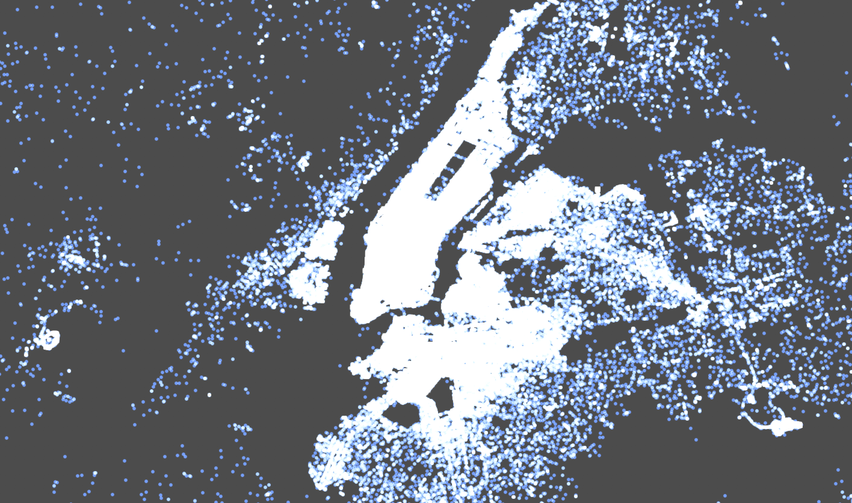
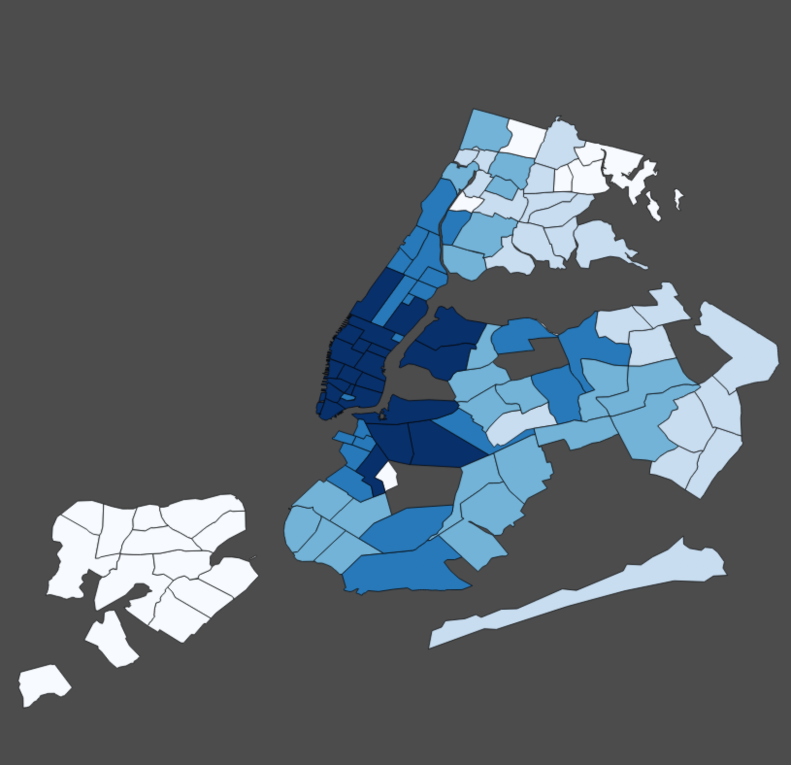
An example of using QGIS and PostGIS to visualize over 700,000 Uber pick-ups. Source: 538 Uber TLC FOIL data.
I've worked for a large ridesharing company for three years. Toward the beginning of my job, I was responsible for much of the public-facing data visualization[1]. Many of my favorite visualizations were static maps, which I've found to be an incredibly useful way of drawing insight from data. Here's a tutorial on how to create works like those using opensource geographic information system (GIS) tooling.
The reasons to use PostGIS are numerous:
Efficiency by avoiding cross-joins. Postgres/PostGIS can index data for hyper-efficient spatial joins. For example, if I have a bunch of polygons for ZIP code boundaries in New York and California, and many points in both California and New York, my query engine should be intelligent enough to determine that it shouldn’t check if a point is contained in an obviously distant shapes–don’t check if points in NY belong in CA.
Scale. You can very easily get about 120 million points indexed on a standard MacBook Pro running PostGIS-- I’m sure you can comfortably get many more on a 2xlarge EC2. (As an added bonus, running these analyses locally means that you don’t have to ask a DBA for permission to make table changes.)
Postgres ecosystem. Postgres is a quite good analytics database, having a rich syntax for date-time handling, analytic functions, custom types, and UDFs, amongst other features.
Living documentation. Since the GIS community has hardly migrated away from PostGIS, you have the benefit of 10+ years of StackOverflow Q+A’s.
QGIS is my vote for the best free geospatial data visualizer and editor. Candidly, I wish I didn’t have to use QGIS. It’s quite buggy--long-time colleagues know I describe it as a piece of malware that happens to double as mapping software. However, it’s still the best free GUI for the job.
- Install Postgres. I'd recommend either Docker PostGIS (if you're familiar with Docker) or the Postgres.app installation if you're not.
- Install PostGIS. Connect to the prompt of your Postgres installation and type
CREATE EXTENSION postgis;If it's already installed, you'll get the messageERROR: extension "postgis" already exists. If instead you see the phraseCREATE EXTENSION, you'll have installed the PostGIS extension for Postgres, which will let us manipulate geometry data in SQL. - Install QGIS. QGIS will help visualize our work. (I recommend the KyngChaos installation if you're using OS X.) It's not uncommon in my experience for QGIS to be buggy, and the installation process is occasionally finicky.
- Install shp2pgsql. You may also need to install shp2pgsql for converting shapefiles to Postgres data.
- Install a basemap plugin. Optional, but highly recommended–install a basemap plugin. This will put a common map (like Google Satellite map or the beautiful Stamen Toner) behind the geometry objects that we’ll visualize.
- From the Uber TLC FOIL data set, download the July 2014 data by right-clicking here and selecting Save as....
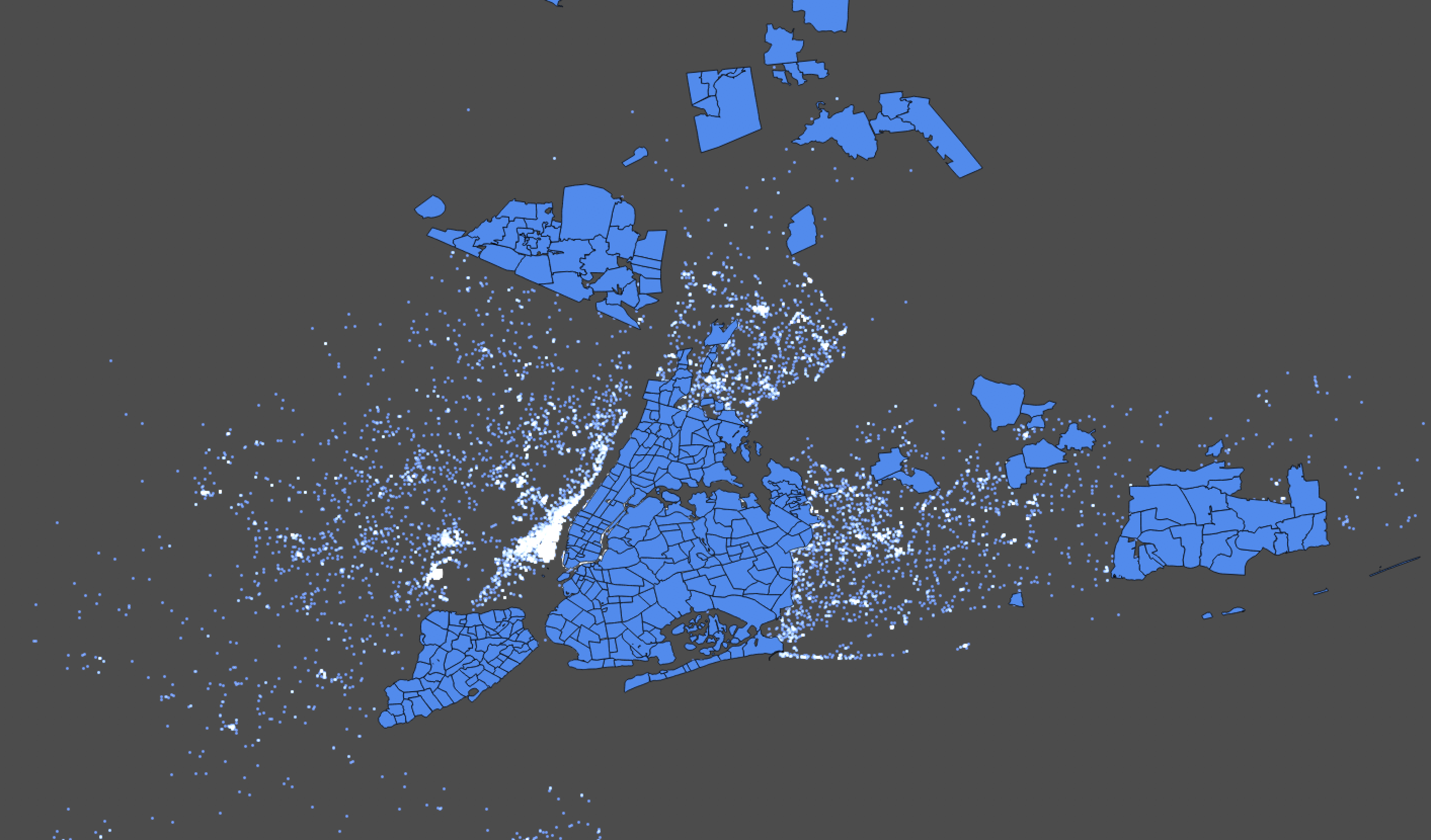
- Download the New York state urban area neighborhood boundaries from Zillow.com by clicking here. Unpack the zip file and double-click on the .shp, and open it up in QGIS. We should be able to navigate to the burroughs of New York City.
Here's a directory with both files:
duberstein@MacBook-Pro:~/Desktop/geo|
⇒  ls
ZillowNeighborhoods-NY  uber-raw-data-jul14.csv
I can copy the neighborhood boundaries into Postgres using the shp2pgsql utility:
duberstein@MacBook-Pro:~/Desktop/geo|
⇒  shp2pgsql -s 4326 ZillowNeighborhoods-NY/ZillowNeighborhoods-NY.shp ny_nbhds postgres > ny.sql
My produces a SQL file with all the shape data--run more ny.sql to see the contents. You can execute that SQL file from psql with the -f flag.
duberstein@MacBook-Pro:~/Desktop/geo|
⇒  psql -f ny.sql
Your psql command may require a different connection string. If you installed Postgres.app, you may want to try,
duberstein@MacBook-Pro:~/Desktop/geo|
⇒  /Applications/Postgres.app/Contents/Versions/9.5/bin/psql -f ny.sql
(If you find yourself typing this frequently and don't want to type this out in full, learn about Bash aliases.)
You've now created a table called ny_nbhds. Check it out using psql:
duberstein@MacBook-Pro:~/Desktop/geo|
⇒  psql
psql (9.5.7)
Type "help" for help.

duberstein=# SELECT COUNT(*) FROM ny_nbhds;
 count
-------
   266
(1 row)
The table itself contains 277 shapes and their metadata:
duberstein=# \x auto
Expanded display is used automatically.
duberstein=# SELECT * FROM ny_nbhds LIMIT 1;
-[ RECORD 1 ]-
gid      | 1
state    | NY
county   | Monroe
city     | Rochester
name     | Ellwanger-Barry
regionid | 343894
geom     | 0106000020E6100...
The shape data in the geom column is represented in a format called well-known binary (WKB), which we'll see a few more times. It's a common representation for geometry data.
We can also see what values are indexed on the table:
duberstein=# \d ny_nbhds
                                     Table "public.ny_nbhds"
  Column  |            Type             |                       Modifiers
----------+-----------------------------+--------------------------------------------------------
 gid      | integer                     | not null default nextval('ny_nbhds_gid_seq'::regclass)
 state    | character varying(2)        |
 county   | character varying(43)       |
 city     | character varying(64)       |
 name     | character varying(64)       |
 regionid | numeric                     |
 geom     | geometry(MultiPolygon,4326) |
Indexes:
    "ny_nbhds_pkey" PRIMARY KEY, btree (gid)
Since we plan to join on geometry data, let's add an index to the geometry like so:
duberstein=# CREATE INDEX ON ny_nbhds USING GIST(geom);
CREATE INDEX
We can use \d again in the psql prompt to verify that we have an additional index:
duberstein=# \d ny_nbhds
                                     Table "public.ny_nbhds"
  Column  |            Type             |                       Modifiers
----------+-----------------------------+--------------------------------------------------------
...
Indexes:
    "ny_nbhds_pkey" PRIMARY KEY, btree (gid)
    "ny_nbhds_geom_idx" gist (geom)
Press ctrl+d to exit psql.
Let's create a table for the points in our CSV. With the head command, we can see the first few lines of data:
duberstein@MacBook-Pro:~/Desktop/geo|
⇒  head uber-raw-data-jul14.csv
"Date/Time","Lat","Lon","Base"
"7/1/2014 0:03:00",40.7586,-73.9706,"B02512"
"7/1/2014 0:05:00",40.7605,-73.9994,"B02512"
"7/1/2014 0:06:00",40.732,-73.9999,"B02512"
...
Back in the psql prompt, we can create a table for this data and then copy it into Postgres:
duberstein@MacBook-Pro:~/Desktop/geo|
⇒  psql
duberstein=# CREATE TABLE uber(datetime TIMESTAMP, lat FLOAT, lng FLOAT, base TEXT);
CREATE TABLE
We've created an empty table called uber.
duberstein=# SELECT * FROM uber;
 datetime | lat | lng | base
----------+-----+-----+------
(0 rows)
We can add data to it from our CSV using psql's \copy command:
duberstein=# \copy uber FROM uber-raw-data-jul14.csv HEADER CSV;
COPY 796121
We've copied 796,121 rows of data from a relative filepath into the uber table. An example of that data
duberstein=# SELECT * FROM uber LIMIT 10;
      datetime       |   lat   |   lng    |  base
---------------------+---------+----------+--------
 2014-07-01 00:03:00 | 40.7586 | -73.9706 | B02512
 2014-07-01 00:05:00 | 40.7605 | -73.9994 | B02512
 2014-07-01 00:06:00 |  40.732 | -73.9999 | B02512
...
(10 rows)
In order to be able to use PostGIS to manipulate this data efficiently, we have to put these lat/lon points in a GEOMETRY data type column.
duberstein=# ALTER TABLE uber ADD COLUMN geom GEOMETRY;
ALTER TABLE
This adds an empty column to each row of data called geom. We can fill that column with an UPDATE command:
duberstein=# UPDATE uber SET geom = ST_SETSRID(ST_POINT(lng, lat), 4326);
UPDATE 796121
A deeper dive into this statement:
-
UPDATEfills thegeomcolumn with the data we feed it after the=. -
ST_POINTreturns a WKB point.ST_SETSRID(..., 4326)sets a value called an spatial reference identifier (SRID) to 4326. Astute readers may have noticed that 4326 has occurred a few times in this document so far. It's a Spatial Reference System Identifier, a way of storing the map projection information about a geometry. You may remember discussions about map projections like Mercator from elementary school--projecting a 3D spheroid like Earth onto a 2D surface like your screen requires encoding some metadata about how that information should be displayed. SRID specifies the encoding for that map projection. What you see on Google Maps and in these examples is 4326, likely the most common map projection. -
You'll also notice that, perhaps unintuitively
lng(our field name for longitude) precedeslat, though we often refer to these points as lat-lon's. Why? Longitude is an X coordinate, and latitude is a Y coordinate, and, if you recall from geometry class, we by convention list coordinates in (X, Y) pairs.
Let's read a few rows of data:
duberstein=# SELECT * FROM uber LIMIT 10;
      datetime       |   lat   |   lng    |  base  |                        geom
---------------------+---------+----------+--------+----------------------------------------------------
 2014-07-01 00:03:00 | 40.7586 | -73.9706 | B02512 | 0101000020E6100000D95F764F1E7E52C0705F07CE19614440
 2014-07-01 00:05:00 | 40.7605 | -73.9994 | B02512 | 0101000020E6100000D5E76A2BF67F52C0D34D621058614440
 2014-07-01 00:06:00 |  40.732 | -73.9999 | B02512 | 0101000020E61000004ED1915CFE7F52C004560E2DB25D4440
 2014-07-01 00:09:00 | 40.7635 | -73.9793 | B02512 | 0101000020E6100000423EE8D9AC7E52C07D3F355EBA614440
 2014-07-01 00:20:00 | 40.7204 | -74.0047 | B02512 | 0101000020E6100000A3923A014D8052C0EA043411365C4440
We've successfully added a GEOMETRY column. Let's index if for efficiency's sake:
duberstein=# CREATE INDEX ON uber USING GIST(geom);
CREATE INDEX
You can run the \d command to verify that the data is indexed, if you'd like.
Open up QGIS. Since the elephant is the official animal of PostgreSQL, click the elephant head on the left panel. Press New to generate a new connection, and add the connection information that's used by psql. If you used Postgres.app, the connection info is as follows:
| Info | Value |
|---|---|
| Host | localhost |
| Port | 5432 |
| User | Your system user name--you can type whoami into a Bash shell to figure this out if it's non-obvious |
| Database | same as user |
| Password | none, leave this blank |
| Connection URL | postgresql://localhost |
Add this connection and save it. Connect to Postgres, and you'll see that we've got tables named uber and ny_nbhds that you can now select and visualize.
Having our pick-up points and neighborhood boundaries loaded into Postgres, we can join the two. Let's count the number of trips by neighbhorhood. In PostGIS, the function for checking a point-in-polygon relationship is ST_Contains. From the PostGIS docs,
ST_Contains — Returns true if and only if no points of B lie in the exterior of A, and at least one point of the interior of B lies in the interior of A.
Less formally, ST_Contains(polygon, point) will return a Boolean, true if the point is within the polygon and false otherwise.
How many points are within the neighborhood boundaries we have?
duberstein=# SELECT COUNT(*) FROM uber u JOIN ny_nbhds n ON ST_CONTAINS(n.geom, u.geom);
 count
--------
 702795
(1 row)
Recall from above that we have 792,121 points in this table, so about 12% of points fall within our neighborhood boundaries. We can use QGIS to visualize this by placing both geometries on a map and visualizing them.
Our data set contains New Jersey-based trips that seem like they'll be excluded in this analysis.
Let's refine our original question: What are the top 10 most frequent neighborhoods for pick-ups? The query below will address that:
SELECT n.name
, COUNT(*) AS freq
FROM uber u
JOIN ny_nbhds n
ON ST_CONTAINS(n.geom, u.geom)
GROUP BY 1
ORDER BY 2 DESC
LIMIT 10
;
The results:
           name            | freq
---------------------------+--------
 Midtown                   | 109671
 Chelsea                   |  55550
 Upper East Side           |  54261
 Gramercy                  |  48617
 Upper West Side           |  35219
 Greenwich Village         |  34716
 Soho                      |  29593
 West Village              |  27678
 Garment District          |  27101
 East Village              |  25890
Let's create a choropleth out of the frequency. We can do this by preserving the result set using a CREATE TABLE ... AS SELECT statement while remembering to include the geometry column from our neighborhood boundaries:
CREATE TABLE pickup_choro AS
SELECT n.name
, n.geom
, COUNT(*) AS freq
FROM uber u
JOIN ny_nbhds n
ON ST_CONTAINS(n.geom, u.geom)
GROUP BY 1, 2
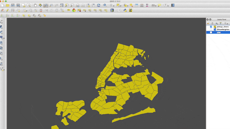
Open up QGIS and select this table. Follow the gif below to style the choropleth.
The end result should look something like this:
[1] For example, here, here, and here.
Neighborhood shapes from Zillow.com used under a Creative Commons Licenese.
538 Uber TLC data obtained by FOIL.