[toc]
-
首先,我們必須知道,test set是用來評估模型推廣到沒看過的data的能力。因此,我們不應該根據test set的結果來調整模型使用的參數。(因為這種修正可能只是對test set的overfitting,面對真正沒看過的data,卻不見得有效。就好像我們已經偷看了答案,看到答案出現很多CCABB,就回去修正我們猜答案的方法一樣。換到另外一張考卷,這種猜法就行不通了。)
-
透過validation set,我們從已知的data中取出一部分來當作調整模型參數的依據,避免根據test set的結果去做調整。(就好像我們拿一些考古題出來,用我們的方法來猜考古題答案,猜得不好的可以做修正,直到找到一個猜得最好的方法,再用他來猜新考題的答案。)
-
但是,根據validation set做的修正,還是有可能只是對valitation set的overfitting。因此,我們必須要增加validation set的變異性。(如果從頭到尾只用一個validation set,就好像每次都看到考古題裡出現CCABB,就把答案背下來。所以,藉由把考古題重新打亂,切成K份,每次只用其中一份做validation,不重複使用,如此做K次,增加變異性,就可避免背答案的狀況。這也就是K-fold Cross Validation的由來。最後選擇K次平均錯誤較低的模型參數,作為最終的模型。)
-
但是,如果data set 是imbalanced,模型就會很容易overfitting到某個答案上去,因此需要將各個答案的數量做平均分配。(例如,我們發現考古題中大量出現C,其他選項ABD都很少,即使做成K-fold 還是大部分只有C。因此,我們將每個fold中的答案比例重新分配,讓ABCD平均出現,這樣每個fold的變異性增加了,就減少背答案的可能。這就是Stratified K-Fold Cross Validation)
-
如果data 數量已經很少,還要拿去做validation就很不經濟了。所以,假設data數量為n,令k=n,將data切成k份,因此每個fold只有一個data,每次只有一個fold=一個data做validation,這就是leave-one-out。(因為考古題數量稀少,所以我們每次只挑一題出來,用我們的模型來猜答案,選擇平均錯誤較低的模型參數,作為最終的模型。)
-
What are training set, validation set and test set?- - 杰 - C++博客
这三个名词在机器学习领域的文章中极其常见,但很多人对他们的概念并不是特别清楚,尤其是后两个经常被人混用。Ripley, B.D(1996)在他的经典专著Pattern Recognition and Neural Networks中给出了这三个词的定义。
Training set: A set of examples used for learning, which is to fit the parameters [i.e., weights] of the classifier.
Validation set: A set of examples used to tune the parameters [i.e., architecture, not weights] of a classifier, for example to choose the number of hidden units in a neural network.
Test set: A set of examples used only to assess the performance [generalization] of a fully specified classifier.
显然,training set是用来训练模型或确定模型参数的,如ANN中权值等; validation set是用来做模型选择(model selection),即做模型的最终优化及确定的,如ANN的结构;而 test set则纯粹是为了测试已经训练好的模型的推广能力。当然,test set这并不能保证模型的正确性,他只是说相似的数据用此模型会得出相似的结果。但实际应用中,一般只将数据集分成两类,即training set 和test set,大多数文章并不涉及validation set。
Ripley还谈到了Why separate test and validation sets?
-
The error rate estimate of the final model on validation data will be biased (smaller than the true error rate) since the validation set is used to select the final model.
-
After assessing the final model with the test set, YOU MUST NOT tune the model any further.
-
-
1.【讨论】如何选择训练集和测试集数据?
一般需要将样本分成独立的三部分训练集(train set),验证集(validation set)和测试集(test set)。其中训练集用来估计模型,验证集用来确定网络结构或者控制模型复杂程度的参数,而测试集则检验最终选择最优的模型的性能如何。一个典型的划分是训练集占总样本的50%,而其它各占25%,三部分都是从样本中随机抽取。
样本少的时候,上面的划分就不合适了。常用的是留少部分做测试集。然后对其余N个样本采用K折交叉验证法。就是将样本打乱,然后均匀分成K份,轮流选择其中K-1份训练,剩余的一份做验证,计算预测误差平方和,最后把K次的预测误差平方和再做平均作为选择最优模型结构的依据。特别的K取N,就是留一法(leave one out)。
-
Cross-Validation in Machine Learning – Towards Data Science
you just can't fit the model to your training data and hope it would accurately work for the real data it has never seen before. You need some kind of assurance that your model has got most of the patterns from the data correct, and its not picking up too much on the noise, or in other words its low on bias and variance.
Generally, an error estimation for the model is made after training, better known as evaluation of residuals. In this process, a numerical estimate of the difference in predicted and original responses is done, also called the training error. However, this only gives us an idea about how well our model does on data used to train it.
So, the problem with this evaluation technique is that it does not give an indication of how well the learner will generalize to an independent/ unseen data set. Getting this idea about our model is known as Cross Validation.
removing a part of the training data and using it to get predictions from the model trained on rest of the data*.*
also known as the holdout method.
it still suffers from issues of high variance. This is because it is not certain which data points will end up in the validation set and the result might be entirely different for different sets.
removing a part of it for validation poses a problem of underfitting. By reducing the training data, we risk losing important patterns/ trends in data set, which in turn increases error induced by bias.
In K Fold cross validation, the data is divided into k subsets. Now the holdout method is repeated k times, such that each time, one of the k subsets is used as the test set/ validation set and the other k-1 subsets are put together to form a training set. The error estimation is averaged over all k trials to get total effectiveness of our model. As can be seen, every data point gets to be in a validation set exactly once, and gets to be in a training set k-1 times. This significantly reduces bias as we are using most of the data for fitting, and also significantly reduces variance as most of the data is also being used in validation set*.*** Interchanging the training and test sets also adds to the effectiveness of this method. As a general rule and empirical evidence, K = 5 or 10 is generally preferred, but nothing's fixed and it can take any value.
In some cases, there may be a large imbalance in the response variables. For example, in dataset concerning price of houses, there might be large number of houses having high price. Or in case of classification, there might be several times more negative samples than positive samples. For such problems, a slight variation in the K Fold cross validation technique is made, such that each fold contains approximately the same percentage of samples of each target class as the complete set, or in case of prediction problems, the mean response value is approximately equal in all the folds*.*** This variation is also known as Stratified K Fold.
Above explained validation techniques are also referred to as Non-exhaustive cross validation methods.
method explained below, also called Exhaustive Methods, that computes all possible ways the data can be split into training and test sets.
This approach leaves p data points out of training data, i.e. if there are n data points in the original sample then, n-p samples are used to train the model and p points are used as the validation set.
This method is exhaustive in the sense that it needs to train and validate the model for all possible combinations, and for moderately large p, it can become computationally infeasible*.*
A particular case of this method is when p = 1. This is known as Leave one out cross validation. This method is generally preferred over the previous one because it does not suffer from the intensive computation, as number of possible combinations is equal to number of data points in original sample or n.
Cross Validation is a very useful technique for assessing the effectiveness of your model, particularly in cases where you need to mitigate overfitting. It is also of use in determining the hyper parameters of your model, in the sense that which parameters will result in lowest test error.
- 從 training data 中取出一部分當作 validation data, validation data取出後不再放回去做training
- 此法的問題在於容易導致較高的變異(variation),因為我們只sample出一部分做validation,但不同sample做validation的差異可能很大,模型訓練時並沒有考慮到這點,最終產出的模型對不同的資料預測結果可能差異很大。
-
將 training data 分割成K份,每次training 只取K-1份,用剩下的一份作validation,每一份都要拿出來做validation,做完一輪共K次。因此,每個資料點只會有一次成為validation set,而有k-1次成為training set。而模型對這個dataset的error由K次validation error的平均來估計。
-
此法可以顯著降低偏差(bias),因為我們充份使用了大部份資料來做training;同時,也會顯著降低變異(variation),因為我們用了大部份資料來做驗證。
-
一般來說,K=5 或 10 是比較合適的
- 當數據不平衡(imbalance)時,將K-Fold中的每個Fold的組成調整成平均分配每個目標分類的樣本數,所以對每個Fold來說,分類結果的數量都幾乎相等。
- 留下p個資料點作驗證,其他n-p做訓練,重複各種可能的組合,共Cn取p次。
- 由於嘗試所有分割的可能,又稱為耗盡法(Exhaustive Methods)。
- 當p很大時,計算量會暴增而變得不可行。
- 因此通常取p=1,又稱為留一法。又可看成 k=n 時的k-Fold。
- 留一法(LOO)通常會造成高變異(variance),因為每次都用n-1個data做training,跟用全部n個data做training是幾乎相同的,無法有效減少變異。
- 所以一般來說,用 K=5 或 10 的K-Fold會比留一法好
| predicted 0 | predicted 1 | |
|---|---|---|
| Actual 0 | True Negative | False Positive |
| Actual 1 | False Negative | True Positive |
-
如何理解与应用调和平均数? - LIQiNG的回答 - 知乎
调和平均数,强调了较小值的重要性;在机器学习中。召回率为R, 准确率为P。使用他们对算法的评估,这两个值通常情况下相互制约。为了更加方便的评价算法的好坏。于是引入了F1值。F1为准确率P和召回率R的调和平均数。为什么F1使用调和平均数,而不是数字平均数。举个例子:当R 接近于1, P 接近于 0 时。采用调和平均数的F1值接近于0;而如果采用算数平均数F1的值为0.5;显然采用调和平均数能更好的评估算法的性能。等效于评价R和P的整体效果
-
准确率(Accuracy), 精确率(Precision), 召回率(Recall)和F1-Measure | ArgCV
有人[3]列了这样个公式, 对非负实数$\beta$ $$ F_\beta=(\beta^2+1)∗ \frac{PR}{\beta^2P+R} $$ 将 F-measure 一般化.
F1-measure 认为精确率和召回率的权重是一样的, 但有些场景下, 我们可能认为精确率会更加重要, 调整参数
$\beta$ , 使用$F_\beta - measure$ 可以帮助我们更好的 evaluate 结果.
-
机器学习中分类器的评价指标:召回率(recall), 精度(precision), 准确率(accuracy), F1分数(F1-score) - liuningjie1119的博客 - CSDN博客
其实多分类的评价指标的计算方式与二分类完全一样,只不过我们计算的是针对于每一类来说的召回率(recall), 精度(precision), 准确率(accuracy)和 F1分数(F1-score).
对于某一个确定的类别来讲,P其实就是实际属于这一类中的样本,N其实就是实际属于其他类的所有样本,P'其实就是被分类器分类这一类的所有样本,N'就是被分类器分类为其他类的所有样本数。
这样来看,对于这一确定的类别来讲,它的召回率(recall)是指被分类器正确分类的属于这个类别的样本数与实际上属于这一类别的总样本数的比值;它的精度(precision)是指被分类器正确分类的属于这个类别的样本数与所有被分类器分为这一类别的样本数的比值。
多分类分类器的准确率/识别率(accuracy)是指所有类别中被分类器分类正确的样本总数与所有样本数的比值。
-
机器学习和统计里面的auc怎么理解? - 现在几点了的回答 - 知乎
从Mann–Whitney U statistic的角度来解释,AUC就是从所有1样本中随机选取一个样本, 从所有0样本中随机选取一个样本,然后根据你的分类器对两个随机样本进行预测,把1样本预测为1的概率为p1,把0样本预测为1的概率为p0,p1>p0的概率就等于AUC
-
ROC空間將偽陽性率(FPR)定義為 X 軸,真陽性率(TPR)定義為 Y 軸。
-
TPR:在所有實際為陽性的樣本中,被正確地判斷為陽性之比率。
-
FPR:在所有實際為陰性的樣本中,被錯誤地判斷為陽性之比率。
給定一個二元分類模型和它的閾值,就能從所有樣本的(陽性/陰性)真實值和預測值計算出一個 (X=FPR, Y=TPR) 座標點。
-


- 如果 sample size 有 unbalanced 的現象可以利用此 accuacy metric 去測量預測精準度 $$ MCC= \frac{TPTN - FPFN}{\sqrt{(TP+FP)(TP+FN)(TN+FP)*(TN+FN)}} $$
-
Machine Learning學習日記 — Coursera篇 (Week 3.4):The – Pandora123 – Medium
What is "overfitting" ?
(1) Overfitting的意思就是太過追求參數完美預測出訓練數據的結果,反而導致實際預測效果不佳
high variance可以理解為其有著過多的 variable
(2) 跟overfit相反的狀況:underfit,代表在訓練數據中也有著高預測誤差的問題
high bias可以理解為其會過度依賴其截距(θ0)
(3) 比較適當的Hypothesis會長的像:
上述都是以Linear Regression為例,下面將以Logistic Regression為例:
Underfit:
Overfit:
而比較剛好的狀況會是
Andrew以一段話談論Overfitting:
If we have too many features, the learned hypothesis may fit the training set very well (J(θ)=0), but fail to generalize to new examples(Predictions on new examples)
那我們要怎麼解決Overfitting的問題呢?
有幾種做法:
1. 降低features的數量:人工選擇、model selection algorithm
2. Regularization:維持現有的features,但是降低部分不重要feature的影響力。這對於有著許多feature的hypothesis很有幫助
下面的例子:左方為適當的模型,右方為Overfitting
我們可以發現主要的問題是在加了θ3跟θ4之後出現了overfitting的問題
那假設我們將θ3跟θ4的影響降到最低呢(讓其逼近於0)?
就像是我們改寫J(θ),多加上1000*(θ3²)和1000*(θ4²)
上述的1000可以隨時替換成一個極大的數值。
而模型自然會為了將J(θ)降到最低,而使θ3跟θ4降至最低,形成下面的粉紅色線構成的模型
以下將舉例說明如何使用Regularization來改善Overfitting的問題
假設我們要預測房價,其包含了很多個features
而我們要做的就是在J(θ)後面加上一個多項式:
這個 λ 其實跟上面例子的數字1000是一樣的意思,它正式的名稱是regularization parameter
按照慣例,這個多項式不會加上截距項θ0
這會大幅改善overfitting的問題
可能會有人好奇 λ 到底代表什麼意思?
λ代表的其實是我們對於預測誤差跟正規項的取捨
當今天 λ越大,模型會比較不重視預測落差反而是極力地想要壓低所有θ值的大小
就像是我們如果把 λ 設成10¹⁰的話,所有θ值都會趨近於0,最後形成一條直線的hypothesis
而若是 λ 越小甚至趨近於0,可能對改善overfitting就沒什麼太大的幫助了
我在學習正規化的時候,對於為什麼只是加上個正規多項式就可以改善overfitting感到非常疑惑
畢竟我們根本不知道要降低哪一個 θ值(feature)的影響力啊
就這樣直接一視同仁的一起打壓所有的θ值到底為什麼會有效?
這是我想到的答案(沒有證實過):的確是一視同仁的打壓所有的 θ值,但是若是今天θ值只要設定到某幾個數字的話可以使預測誤差降到非常低的話,那麼模型如果為了貪小便宜的將那幾個 θ值給壓低反而造成了預測誤差的大幅上升,使得J(θ)不降反升的反效果的話,會非常得不償失,因此模型將會斟酌不要降低那些重要的 θ值
上述的假設都建立在今天 λ 設立得宜的情況以及有足夠的資料來support預測落差的下降,說服模型不要把重要的 θ值降低


-
Regularization in Machine Learning – Towards Data Science
A simple relation for linear regression looks like this. Here Y represents the learned relation and β represents the coefficient estimates for different variables or predictors(X).
Y ≈ β0 + β1X1 + β2X2 + ...+ βpXp
The fitting procedure involves a loss function, known as residual sum of squares or RSS. The coefficients are chosen, such that they minimize this loss function.
Now, this will adjust the coefficients based on your training data. If there is noise in the training data, then the estimated coefficients won't generalize well to the future data. This is where regularization comes in and shrinks or regularizes these learned estimates towards zero.
Above image shows ridge regression, where the RSS is modified by adding the shrinkage quantity. Now, the coefficients are estimated by minimizing this function. Here, λ is the tuning parameter that decides how much we want to penalize the flexibility of our model.
When λ = 0, the penalty term has no effect, and the estimates produced by ridge regression will be equal to least squares. However, as λ→∞, the impact of the shrinkage penalty grows, and the ridge regression coefficient estimates will approach zero. As can be seen, selecting a good value of λ is critical. Cross validation comes in handy for this purpose. The coefficient estimates produced by this method are also known as the L2 norm.
The coefficients that are produced by the standard least squares method are scale equivariant, i.e. if we multiply each input by c then the corresponding coefficients are scaled by a factor of 1/c. Therefore, regardless of how the predictor is scaled, the multiplication of predictor and coefficient(Xjβj) remains the same. However, this is not the case with ridge regression, and therefore, we need to standardize the predictors or bring the predictors to the same scale before performing ridge regression. The formula used to do this is given below.
Lasso is another variation, in which the above function is minimized. Its clear that this variation differs from ridge regression only in penalizing the high coefficients. It uses |βj|(modulus)instead of squares of β, as its penalty. In statistics, this is** known as the L1 norm**.
Consider their are 2 parameters in a given problem. Then according to above formulation, the ridge regression is expressed by β1² + β2² ≤ s. This implies that ridge regression coefficients have the smallest RSS(loss function) for all points that lie within the circle given by β1² + β2² ≤ s.
Similarly, for lasso, the equation becomes,|β1|+|β2|≤ s. This implies that lasso coefficients have the smallest RSS(loss function) for all points that lie within the diamond given by |β1|+|β2|≤ s.
The image below describes these equations.
Credit : An Introduction to Statistical Learning by Gareth James, Daniela Witten, Trevor Hastie, Robert Tibshirani
The above image shows the constraint functions(green areas), for lasso(left) and ridge regression(right), along with contours for RSS(red ellipse). Points on the ellipse share the value of RSS. For a very large value of s, the green regions will contain the center of the ellipse, making coefficient estimates of both regression techniques, equal to the least squares estimates. But, this is not the case in the above image. In this case, the lasso and ridge regression coefficient estimates are given by the first point at which an ellipse contacts the constraint region. Since ridge regression has a circular constraint with no sharp points, this intersection will not generally occur on an axis, and so the ridge regression coefficient estimates will be exclusively non-zero.** However, the lasso constraint has corners at each of the axes, and so the ellipse will often intersect the constraint region at an axis. When this occurs, one of the coefficients will equal zero.** In higher dimensions(where parameters are much more than 2), many of the coefficient estimates may equal zero simultaneously.
Therefore, the lasso method also performs variable selection and is said to yield sparse models.
Regularization, significantly reduces the variance of the model, without substantial increase in its bias.
As the value of λ rises, it reduces the value of coefficients and thus reducing the variance.
But after certain value, the model starts loosing important properties, giving rise to bias in the model and thus underfitting.
總結:
L2 norm 就是把所有係數取平方和乘上λ後最小化
L1 norm 就是把所有係數取絕對值乘上λ後最小化
以兩個係數β1,β2為例,
L2 norm 可以寫成β1^2 + β2^2 <=s,因此是個圓形區域,參數收斂到最後會碰到圓形區域的邊界,因此通常兩個係數都不會是0 L1 norm 可以寫成|β1| + |β2| <=s,因此是個菱形區域,參數收斂到最後會碰到菱形的尖點上,由於此點在座標軸上,因此會產生其他座標軸係數為0的效果,可用來篩選不重要的特徵。
Regularization 正則化可以顯著降低參數的 variance,而不增加bias;然而,當λ超過某個數值後,就會變成underfitting。因此需要慎選λ。而 cross validation 就是用來做這件事。 [name=Ya-Lun Li]


-
實作Tensorflow (4):Autoencoder - YC Note
以下的Regularizer不是採用單純的L2 Regularizer,我將會使用Weight-Elimination L2 Regularizer,這個Regularizer的好處是會使得權重接近Sparse,也就是說權重會留下比較多的0,這有一個好處,就是每個神經元彼此之間的依賴減少了,因為內積(評估相依性)時有0的那個維度將不會有所貢獻。
Weight-Elimination L2 Regularizer有這樣的效果原因是這樣的,L2 Regularizer在抑制W的方法是,如果$W$的分量大的話就抑制多一點,如果分量小就抑制少一點(因為$W^2$微分為一次),所以最後會留下很多不為0的微小分量,不夠Sparse,這樣的Regularization顯然不夠好,L1 Regularizer可以解決這個問題(因為在大部分位置微分為常數),但不幸的是它無法微分,沒辦法作Backpropagation,所以就有了L2 Regularizer的衍生版本,Weight-elimination L2 regularizer:
$$\sum_{jk} (W_{jk} (ℓ))^2 / [1+ (W_{jk} (ℓ) )^2]$$ 這麼一來不管W大或小,它受到抑制的值大小接近的 (Weight-elimination L2 regularizer微分為
$-1$ 次方),因此就可以使得部分$W$可以為$0$,達成Sparse的目的。那為什麼我要特別在Autoencoder講究Sparse特性呢?原因是我們現在正在做的事是Dimension Reduction,做這件事就好像是替原本空間找出新的軸,而這個軸的數量比原本空間軸的數量來得小,達到Dimension Reduction的效果,所以我們會希望這個新的軸彼此間可以不要太多的依賴,什麼是不依賴呢?直角座標就是最不依賴的座標系,X軸和Y軸內積為0,這樣的軸展開的效率是最好的,所以我們希望在做Regularization的同時可以減少新軸的彼此間的依賴性。

-
這項研究,就是加州大學伯克利分校和MIT的幾名科學家在arXiv上公開的一篇論文:Do CIFAR-10 Classifiers Generalize to CIFAR-10?。
解釋一下,這個看似詭異的問題——「CIFAR-10分類器能否泛化到CIFAR-10?」,針對的是當今深度學習研究的一個大缺陷:
看起來成績不錯的深度學習模型,在現實世界中不見得管用。因爲很多模型和訓練方法取得的好成績,都來自對於那些著名基準驗證集的過擬合。
-
常用測試集帶來過擬合?你真的能控制自己不根據測試集調參嗎 - 幫趣
儘管對比新模型與之前模型的結果是非常自然的想法,但很明顯當前的研究方法論削弱了一個關鍵假設:分類器與測試集是獨立的。這種不匹配帶來了一種顯而易見的危險,研究社區可能會輕易設計出只在特定測試集上性能良好,但無法泛化至新數據的模型 [1]。
該研究分爲三步:
-
首先,研究者創建一個新的測試集,將新測試集的子類別分佈與原始 CIFAR-10 數據集進行仔細匹配。
-
在收集了大約 2000 張新圖像之後,研究者在新測試集上評估 30 個圖像分類模型的性能。結果顯示出兩個重要現象。一方面,從原始測試集到新測試集的模型準確率顯著下降。例如,VGG 和 ResNet 架構 [7, 18] 的準確率從 93% 下降至新測試集上的 85%。另一方面,研究者發現在已有測試集上的性能可以高度預測新測試集上的性能。即使在 CIFAR-10 上的微小改進通常也能遷移至留出數據。
-
受原始準確率和新準確率之間差異的影響,第三步研究了多個解釋這一差距的假設。一種自然的猜想是重新調整標準超參數能夠彌補部分差距,但是研究者發現該舉措的影響不大,僅能帶來大約 0.6% 的改進。儘管該實驗和未來實驗可以解釋準確率損失,但差距依然存在。
總之,研究者的結果使得當前機器學習領域的進展意味不明。適應 CIFAR-10 測試集的努力已經持續多年,模型表現的測試集適應性並沒有太大提升。頂級模型仍然是近期出現的使用 Cutout 正則化的 Shake-Shake 網絡 [3, 4]。此外,該模型比標準 ResNet 的優勢從 4% 上升至新測試集上的 8%。這說明當前對測試集進行長時間「攻擊」的研究方法具有驚人的抗過擬合能力。
但是該研究結果令人對當前分類器的魯棒性產生質疑。儘管新數據集僅有微小的分佈變化,但廣泛使用的模型的分類準確率卻顯著下降。例如,前面提到的 VGG 和 ResNet 架構,其準確率損失相當於模型在 CIFAR-10 上的多年進展 [9]。注意該實驗中引入的分佈變化不是對抗性的,也不是不同數據源的結果。因此即使在良性設置中,分佈變化也對當前模型的真正泛化能力帶來了嚴峻挑戰。
-
-
Tomaso Poggio深度學習理論:深度網絡「過擬合缺失」的本質 - 幫趣
本文是 DeepMind 創始人 Demis Hassabis 和 Mobileye 創始人 Amnon Shashua 的導師、MIT 教授 Tomaso Poggio 的深度學習理論系列的第三部分,分析深度神經網絡的泛化能力。該系列前兩部分討論了深度神經網絡的表徵和優化問題,機器之心之前對整個理論系列進行了簡要總結。在深度網絡的實際應用中,通常會添加顯性(如權重衰減)或隱性(如早停)正則化來避免過擬合,但這並非必要,尤其是在分類任務中。在本文中,Poggio 討論了深度神經網絡的過擬合缺失問題,即在參數數量遠遠超過訓練樣本數的情況下模型也具備良好的泛化能力。其中特別強調了經驗損失和分類誤差之間的差別,證明深度網絡每一層的權重矩陣可收斂至極小范數解,並得出深度網絡的泛化能力取決於多種因素的互相影響,包括損失函數定義、任務類型、數據集類型等。
1 引言
過去幾年來,深度學習在許多機器學習應用領域都取得了極大的成功。然而,我們對深度學習的理論理解以及開發原理的改進能力上都有所落後。如今對深度學習令人滿意的理論描述正在形成。這涵蓋以下問題:1)深度網絡的表徵能力;2)經驗風險的優化;3)泛化------當網絡過參數化(overparametrized)時,即使缺失顯性的正則化,爲什麼期望誤差沒有增加?
本論文解決了第三個問題,也就是非過擬合難題,這在最近的多篇論文中都有提到。論文 [1] 和 [7] 展示了線性網絡的泛化特性可被擴展到 DNN 中從而解決該難題,這兩篇論文中的泛化即用梯度下降訓練的帶有特定指數損失的線性網絡收斂到最大間隔解,提供隱性的正則化。本論文還展示了同樣的理論可以預測經驗風險的不同零最小值(zero minimizer)的泛化。
2 過擬合難題
經典的學習理論將學習系統的泛化行爲描述爲訓練樣本數 n 的函數。從這個角度看,DNN 的行爲和期望一致:更多訓練數據帶來更小的測試誤差,如圖 1a 所示。該學習曲線的其他方面似乎不夠直觀,但也很容易解釋。例如即使在訓練誤差爲零時,測試誤差也會隨着 n 的增加而減小(正如 [1] 中所指出的那樣,因爲被報告的是分類誤差,而不是訓練過程中被最小化的風險,如交叉熵)。看起來 DNN 展示出了泛化能力,從技術角度上可定義爲:隨着 n → ∞,訓練誤差收斂至期望誤差。圖 1 表明對於正常和隨機標籤,模型隨 n 的增加的泛化能力變化。這與之前研究的結果一致(如 [8]),與 [9] 的穩定性結果尤其一致。注意泛化的這一特性並不尋常:很多算法(如 K 最近鄰算法)並不具備該保證。
圖 1:不同數量訓練樣本下的泛化。(a)在 CIFAR 數據集上的泛化誤差。(b)在隨機標籤的 CIFAR 數據集上的泛化誤差。該深度神經網絡是通過最小化交叉熵損失訓練的,並且是一個 5 層卷積網絡(即沒有池化),每個隱藏層有 16 個通道。ReLU 被用做層之間的非線性函數。最終的架構有大約 1 萬個參數。圖中每一個點使用批大小爲 100 的 SGD 並訓練 70 個 epoch 而得出,訓練過程沒有使用數據增強和正則化。
泛化的這一特性雖然重要,但在這裏也只是學術上很重要。現在深度網絡典型的過參數化真正難題(即本論文的重點)是在缺乏正則化的情況下出現明顯缺乏過擬合的現象。從隨機標註數據中獲得零訓練誤差的同樣網絡(圖 1b)很顯然展示出了大容量,但並未展示出在不改變多層架構的情況下,每一層神經元數量增加時期望誤差會有所增加(圖 2a)。具體來說,當參數數量增加並超過訓練集大小時,未經正則化的分類誤差在測試集上的結果並未變差。
圖 2:在 CIFAR-10 中的期望誤差,橫軸爲神經元數量。該 DNN 與圖 1 中的 DNN 一樣。(a)期望誤差與參數數量增加之間的相關性。(b)交叉熵風險與參數數量增加之間的相關性。期望風險中出現部分「過擬合」,儘管該指數損失函數的特點略微有些誇大。該過擬合很小,因爲 SGD 收斂至每一層具備最小弗羅貝尼烏斯範數(Frobenius norm)的網絡。因此,當參數數量增加時,這裏的期望分類誤差不會增加,因爲分類誤差比損失具備更強的魯棒性(見附錄 9)。
我們應該明確參數數量只是過參數化的粗略表徵。實驗設置詳見第 6 章。
5 深度網絡的非線性動態
5.3 主要問題
把所有引理合在一起,就得到了
定理 3:給定一個指數損失函數和非線性分割的訓練數據,即對於訓練集中的所有 x_n,∃f(W; x_n) 服從 y_n*f(W; x_n) > 0,獲得零分類誤差。以下特性展示了漸近平衡(asymptotic equilibrium):
-
GD 引入的梯度流從拓撲學角度來看等於線性化流;
-
解是每一層權重矩陣的局部極小弗羅貝尼烏斯範數解。
在平方損失的情況下分析結果相同,但是由於線性化動態只在零初始條件下收斂至極小范數,因此該定理的最終表述「解是局部極小範數解」僅適用於線性網絡,如核機器,而不適用於深度網絡。因此在非線性的情況下,平方損失和指數損失之間的差別變得非常顯著。對其原因的直觀理解見圖 3。對於全局零最小值附近的深度網絡,平方損失的「地形圖」通常有很多零特徵值,且在很多方向上是平坦的。但是,對於交叉熵和其他指數損失而言,經驗誤差山谷有一個很小的向下的坡度,在||w||無限大時趨近於零(詳見圖 3)。
在補充材料中,研究者展示了通過懲罰項 λ 寫出 W_k = ρ_k*V_k,並使 ||V_k||^2 = 1,來考慮相關動態,從而展示初始條件的獨立性以及早停和正則化的等效性。
圖 3:具備參數 w_1 和 w_2 的平方損失函數(左)。極小值具備一個退化 Hessian(特徵值爲零)。如文中所述,它表示在零最小值的小近鄰區域的「一般」情況,零最小值具備很多零特徵值,和針對非線性多層網絡的 Hessian 的一些正特徵值。收斂處的全局最小值附近的交叉熵風險圖示如右圖所示。隨着||w|| → ∞,山谷坡度稍微向下。在多層網絡中,損失函數可能表面是分形的,具備很多退化全局最小值,每個都類似於這裏展示的兩個最小值的多維度版本。
5.4 爲什麼分類比較不容易過擬合
由於這個解是線性化系統的極小範數解,因此我們期望,對於低噪聲數據集,與交叉熵最小化相關的分類誤差中幾乎很少或沒有過擬合。注意:交叉熵作爲損失函數的情況中,梯度下降在線性分離數據上可收斂至局部極大間隔解(local max-margin solution),起點可以是任意點(原因是非零斜率,如圖 3 所示)。因此,對於期望分類誤差,過擬合可能根本就不會發生,如圖 2 所示。通常相關損失中的過擬合很小,至少在幾乎無噪聲的數據情況下是這樣,因爲該解是局部極大間隔解,即圍繞極小值的線性化系統的僞逆。近期結果(Corollary 2.1 in [10])證明具備 RELU 激活函數的深度網絡的 hinge-loss 的梯度最小值具備大的間隔,前提是數據是可分離的。這個結果與研究者將 [1] 中針對指數損失的結果擴展至非線性網絡的結果一致。注意:目前本論文研究者沒有對期望誤差的性質做出任何聲明。不同的零最小值可能具備不同的期望誤差,儘管通常這在 SGD 的類似初始化場景中很少出現。本文研究者在另一篇論文中討論了本文提出的方法或許可以預測與每個經驗最小值相關的期望誤差。
總之,本研究結果表明多層深度網絡的行爲在分類中類似於線性模型。更準確來說,在分類任務中,通過最小化指數損失,可確保全局最小值具備局部極大間隔。因此動態系統理論爲非過擬合的核心問題提供了合理的解釋,如圖 2 所示。主要結果是:接近經驗損失的零極小值,非線性流的解繼承線性化流的極小範數特性,因爲這些流拓撲共軛。損失中的過擬合可以通過正則化來顯性(如通過權重衰減)或隱性(通過早停)地控制。分類誤差中的過擬合可以被避免,這要取決於數據集類型,其中漸近解是與特定極小值相關的極大間隔解(對於交叉熵損失來說)。
6 實驗
圖 4:使用平方損失在特徵空間中對線性網絡進行訓練和測試(即 y = WΦ(X)),退化 Hessian 如圖 3 所示。目標函數是一個 sine 函數 f(x) = sin(2πfx),在區間 [-1, 1] 上 frequency f = 4。訓練數據點有 9 個,而測試數據點的數量是 100。第一對圖中,特徵矩陣 φ(X) 是多項式的,degree 爲 39。第一對圖中的數據點根據 Chebyshev 節點機制進行採樣,以加速訓練,使訓練誤差達到零。訓練使用完整梯度下降進行,步長 0.2,進行了 10, 000, 000 次迭代。每 120, 000 次迭代後權重受到一定的擾動,每一次擾動後梯度下降被允許收斂至零訓練誤差(機器準確率的最高點)。通過使用均值 0 和標準差 0.45 增加高斯噪聲,進而擾動權重。在第 5, 000, 000 次迭代時擾動停止。第二張圖展示了權重的 L_2 範數。注意訓練重複了 29 次,圖中報告了平均訓練和測試誤差,以及權重的平均範數。第二對圖中,特徵矩陣 φ(X) 是多項式的,degree 爲 30。訓練使用完整梯度下降進行,步長 0.2,進行了 250, 000 次迭代。第四張圖展示了權重的 L_2 範數。注意:訓練重複了 30 次,圖中報告了平均訓練和測試誤差,以及權重的平均範數。該實驗中權重沒有遭到擾動。
7 解決過擬合難題
本研究的分析結果顯示深度網絡與線性模型類似,儘管它們可能過擬合期望風險,但不經常過擬合低噪聲數據集的分類誤差。這遵循線性網絡梯度下降的特性,即風險的隱性正則化和對應的分類間隔最大化。在深度網絡的實際應用中,通常會添加顯性正則化(如權重衰減)和其他正則化技術(如虛擬算例),而且這通常是有益的,雖然並非必要,尤其是在分類任務中。
如前所述,平方損失與指數損失不同。在平方損失情況中,具備任意小的 λ 的正則化(沒有噪聲的情況下)保留梯度系統的雙曲率,以收斂至解。但是,解的範數依賴於軌跡,且無法確保一定會是線性化引入的參數中的局部極小範數解(在非線性網絡中)。在沒有正則化的情況下,可確保線性網絡(而不是深度非線性網絡)收斂至極小范數解。在指數損失線性網絡和非線性網絡的情況下,可獲得雙曲梯度流。因此可確保該解是不依賴初始條件的極大間隔解。對於線性網絡(包括核機器),存在一個極大間隔解。在深度非線性網絡中,存在多個極大間隔解,每個對應一個全局最小值。在某種程度上來說,本研究的分析結果顯示了正則化主要提供了動態系統的雙曲率。在條件良好的線性系統中,即使 λ → 0,這種結果也是對的,因此內插核機器的通用情況是在無噪聲數據情況下無需正則化(即條件數依賴於 x 數據的分割,因此 y 標籤與噪聲無關,詳見 [19])。在深度網絡中,也會出現這種情況,不過只適用於指數損失,而非平方損失。
結論就是深度學習沒什麼神奇,在泛化方面深度學習需要的理論與經典線性網絡沒什麼不同,泛化本身指收斂至期望誤差,尤其是在過參數化時出現了過擬合缺失的情況。本研究分析通過將線性網絡的特性(如 [1] 強調的那些)應用到深度網絡,解釋了深度網絡泛化方面的難題,即不會過擬合期望分類誤差。
8 討論
當然,構建對深度網絡性能有用的量化邊界仍然是一個開放性問題,因爲它是非常常見的情形,即使是對於簡單的僅包含一個隱藏層的網絡,如 SVM。本論文研究者主要的成果是圖 2 所展示的令人費解的行爲可以通過經典理論得到定性解釋。
該領域存在很多開放性問題。儘管本文解釋了過擬合的缺失,即期望誤差對參數數量增加的容錯,但是本文並未解釋爲什麼深度網絡泛化得這麼好。也就是說,本論文解釋了爲什麼在參數數量增加並超過訓練數據數量時,圖 2 中的測試分類誤差沒有變差,但沒有解釋爲什麼測試誤差這麼低。
基於 [20]、[18]、[16]、[10],研究者猜測該問題的答案包含在以下深度學習理論框架內:
-
不同於淺層網絡,深度網絡能逼近層級局部函數類,且不招致維數災難([21, 20])。
-
經由 SGD 選擇,過參數化的深度網絡有很大概率會產生很多全局退化,或者大部分退化,以及「平滑」極小值([16])。
-
過參數化,可能會產生預期風險的過擬合。因爲梯度下降方法獲得的間隔最大化,過參數化也能避免過擬合低噪聲數據集的分類誤差。
根據這一框架,淺層網絡與深度網絡之間的主要區別在於,基於特定任務的組織結構,兩種網絡從數據中學習較好表徵的能力,或者說是逼近能力。不同於淺層網絡,深度局部網絡特別是卷積網絡,能夠避免逼近層級局部合成函數類時的維度災難(curse of dimensionality)。這意味着對於這類函數,深度局部網絡可以表徵一種適當的假設類,其允許可實現的設置,即以最小容量實現零逼近誤差。
論文:Theory IIIb: Generalization in Deep Networks
論文鏈接:https://arxiv.org/abs/1806.11379
**摘要:**深度神經網絡(DNN)的主要問題圍繞着「過擬合」的明顯缺失,本論文將其定義如下:當神經元數量或梯度下降迭代次數增加時期望誤差卻沒有變差。鑑於 DNN 擬合隨機標註數據的大容量和顯性正則化的缺失,這實在令人驚訝。近期 Srebro 等人的研究結果爲二分類線性網絡中的該問題提供瞭解決方案。他們證明損失函數(如 logistic、交叉熵和指數損失)最小化可在線性分離數據集上漸進、「緩慢」地收斂到最大間隔解,而不管初始條件如何。本論文中我們證明了對於非線性多層 DNN 在經驗損失最小值接近零的情況下也有類似的結果。指數損失的結果也是如此,不過不適用於平方損失。具體來說,我們證明深度網絡每一層的權重矩陣可收斂至極小范數解,達到比例因子(在獨立案例下)。我們對動態系統的分析對應多層網絡的梯度下降,這展示了一種對經驗損失的不同零最小值泛化性能的簡單排序標準。
-
-
深度神經網絡爲什麼不易過擬合?傅里葉分析發現固有頻譜偏差 - 幫趣
-
本文展示了對於參數 θ 的任意有限值來說,深度神經網絡(DNN)的 ReLU 函數的一個特定的頻率分量(k)的量級至少以 O(1/k^2 ) 的速率衰減,並且網絡的寬度和深度分別以多項式和指數的級別幫助其捕獲更高的頻率;因此,高頻分量的大小會更小(DNN 更容易趨向於光滑)。其結果是,對深度神經網絡(DNN)進行有限步訓練使其更趨向於表示如上面所描述的函數。
-
作爲這一理論的附帶結果,研究者揭示了(有限權重)深度神經網絡在學習類似狄拉克 delta 函數(單位脈衝函數)峯函數的理論極限。這是因爲它的傅立葉變換的量級是一個常值函數(因此所有的頻率都有相同的振幅)。並且如上文中所討論的,深度神經網絡(DNN)無法學習對這樣的函數建模,因爲它們的傅立葉係數必須至少以 1/k^2 的速率衰減(儘管增加寬度和深度可以分別以多項式級和指數級別幫助其捕獲更高的頻率)。
-
研究者指出,如果在低維流形上定義數據-目標函數的映射,深度神經網絡(DNN)可以利用流形的幾何結構來對函數取近似,這些函數沿着流形(其函數的頻率分量相對於其輸入空間較低)具有高頻分量。
-
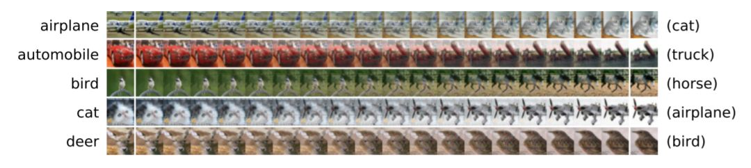
通過分析實驗表明,對於一個在 CIFAR-10 數據集上訓練的深度神經網絡(DNN)來說,存在幾乎線性的路徑能夠連接所有的對抗性樣本,它們被分類成一個特定的類(比如「貓」)。對於所有真正類別爲「貓」的訓練樣本,所有的樣本也沿着這條路徑被分類成同一個類別------「貓」。研究者進一步展示了對於在 CIFAR-10 數據集上訓練的深度神經網絡(DNN)來說,所有同一個類別中的訓練樣本也通過同樣的方式連接起來。
-
實驗表明,與帶有高頻分量的函數相對應的深度神經網絡(DNN)在參數空間中所佔的體積更小。
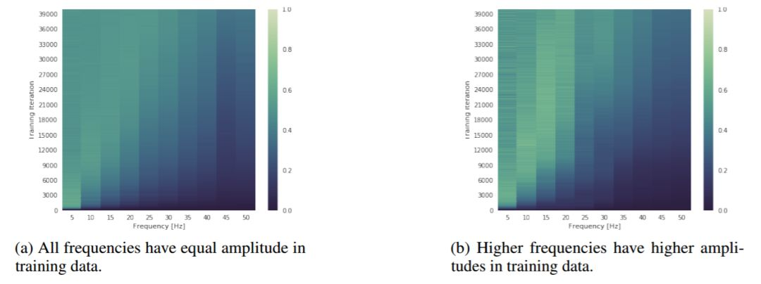
圖 2:展示訓練期間(y 軸)頻譜演變(x 軸)的熱圖。顏色代表測量出的在相應的頻率上網絡頻譜的幅值,其值用相同的頻率的目標幅值進行了歸一化操作。此圖說明,儘管更高頻率的訓練數據具有 g 的振幅,深度神經網絡仍然優先訓練低頻數據。
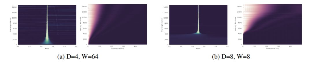
圖 3: 一個深度爲 D、寬度爲 W,權重修剪 K=0.1 的網絡被訓練去預測一個 delta 峯(所有頻率的振幅都相同)。在圖(a)和圖(b)中,y 軸對應於不斷增加的訓練迭代次數(向上遞增),x 軸則代表頻域(右圖)和輸入域(左圖)。更亮的顏色表示數值更大。此圖說明,根據理論所闡述的,寬度和深度分別以多項式和指數級幫助網絡捕獲高頻分量。這一點在輸入域和頻域上都可以看出來(注:64^4=8^8)。更多的圖片請參見附錄(圖 11)。
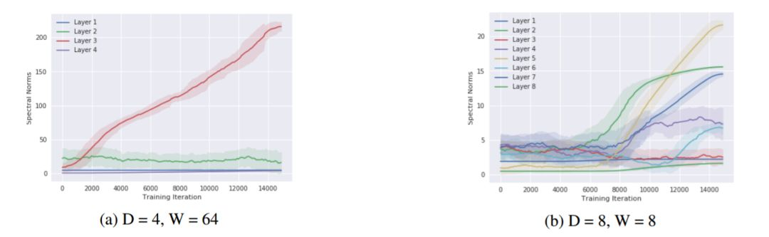
圖 5: 在圖 3 中所使用的 delta 峯數據集上,一個深度爲 D 層、寬度爲 W 個單元的網絡的所有權重的譜範數(y 軸)與訓練過程中迭代次數(x 軸)的關係圖。
對於矩陣值權重,它們的譜範數是通過估計由 10 次冪迭代得到的特徵向量的特徵值計算而來。對於向量值權重,則僅使用了 L2 範數。此圖說明,隨着神經網絡通過學習去擬合更大的頻率,神經網絡權值的譜範數也增大,從而鬆弛頻譜的邊界
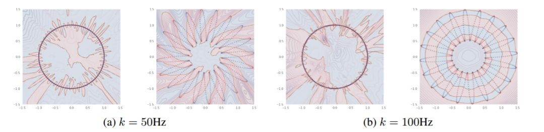
圖 6: 在圖(a)和圖(b)中,左圖:L=0 瓣(虛線圓);右圖:L=20 瓣(由 20 瓣組成的虛線花)定義了數據的流形。
對於這兩個流形,我們沿着流形定義了一個頻率爲 k Hz 的正弦信號,並將它二值化,得到一個 0/1 的目標(點的顏色)。對於每種情況,研究者訓練了一個 6 層深的 ReLU 網絡,將數據樣本從流形映射到它相應的目標上。填充的顏色表示預測出的類,等高線表示該網絡經過 sigmoid 函數處理的對數 logits 的絕對值。此圖說明,對應較大的 L 的流形,即使在兩種流形沿着流形的目標頻率相同時,也能使深度神經網絡在其域空間學習到更光滑的函數。可以看到,網絡會學習利用 L 值較大的流形的幾何結構去學習關於其輸入空間的低頻函數。這個結論在另一個實驗中得到了證實。
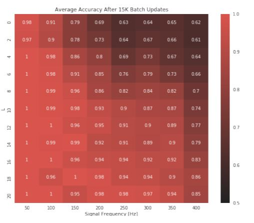
圖 8: 用於預測定義在一個 L 瓣的流形(y 軸)上的給定頻率(x 軸)的二值化正弦波的訓練分類準確率的熱圖。此圖說明,如果目標信號的頻率較低或數據定義在一個具有更大的 L 的流形上,固定大小的網絡的準確率越高。後者的結果表明,隨着流形中瓣數的增加,在一個流形上學習一個高頻目標就變得更容易。
圖 9: 每一行都展示了圖像空間中的一條路徑,從右至左顯示了從對抗性樣本變爲一個真實訓練圖像的過程。
-


-
Classification when 80% of my training set is of one class.:MachineLearning
-
In classification, how do you handle an unbalanced training set? - Quora
-
8 Tactics to Combat Imbalanced Classes in Your Machine Learning Dataset
You might think it's silly, but collecting more data is almost always overlooked.
Can you collect more data? Take a second and think about whether you are able to gather more data on your problem.
A larger dataset might expose a different and perhaps more balanced perspective on the classes.
More examples of minor classes may be useful later when we look at resampling your dataset.
Accuracy is not the metric to use when working with an imbalanced dataset. We have seen that it is misleading.
There are metrics that have been designed to tell you a more truthful story when working with imbalanced classes.
I give more advice on selecting different performance measures in my post "Classification Accuracy is Not Enough: More Performance Measures You Can Use".
In that post I look at an imbalanced dataset that characterizes the recurrence of breast cancer in patients.
From that post, I recommend looking at the following performance measures that can give more insight into the accuracy of the model than traditional classification accuracy:
- Confusion Matrix: A breakdown of predictions into a table showing correct predictions (the diagonal) and the types of incorrect predictions made (what classes incorrect predictions were assigned).
- Precision: A measure of a classifiers exactness.
- Recall: A measure of a classifiers completeness
- F1 Score (or F-score): A weighted average of precision and recall.
I would also advice you to take a look at the following:
- Kappa (or Cohen's kappa): Classification accuracy normalized by the imbalance of the classes in the data.
- ROC Curves: Like precision and recall, accuracy is divided into sensitivity and specificity and models can be chosen based on the balance thresholds of these values.
You can learn a lot more about using ROC Curves to compare classification accuracy in our post "Assessing and Comparing Classifier Performance with ROC Curves".
Still not sure? Start with kappa, it will give you a better idea of what is going on than classification accuracy.
You can change the dataset that you use to build your predictive model to have more balanced data.
This change is called sampling your dataset and there are two main methods that you can use to even-up the classes:
- You can add copies of instances from the under-represented class called over-sampling (or more formally sampling with replacement), or
- You can delete instances from the over-represented class, called under-sampling.
These approaches are often very easy to implement and fast to run. They are an excellent starting point.
In fact, I would advise you to always try both approaches on all of your imbalanced datasets, just to see if it gives you a boost in your preferred accuracy measures.
You can learn a little more in the the Wikipedia article titled "Oversampling and undersampling in data analysis".
- Consider testing under-sampling when you have an a lot data (tens- or hundreds of thousands of instances or more)
- Consider testing over-sampling when you don't have a lot of data (tens of thousands of records or less)
- Consider testing random and non-random (e.g. stratified) sampling schemes.
- Consider testing different resampled ratios (e.g. you don't have to target a 1:1 ratio in a binary classification problem, try other ratios)
A simple way to generate synthetic samples is to randomly sample the attributes from instances in the minority class.
You could sample them empirically within your dataset or you could use a method like Naive Bayes that can sample each attribute independently when run in reverse. You will have more and different data, but the non-linear relationships between the attributes may not be preserved.
There are systematic algorithms that you can use to generate synthetic samples. The most popular of such algorithms is called SMOTE or the Synthetic Minority Over-sampling Technique.
As its name suggests, SMOTE is an oversampling method. It works by creating synthetic samples from the minor class instead of creating copies. The algorithm selects two or more similar instances (using a distance measure) and perturbing an instance one attribute at a time by a random amount within the difference to the neighboring instances.
Learn more about SMOTE, see the original 2002 paper titled "SMOTE: Synthetic Minority Over-sampling Technique".
There are a number of implementations of the SMOTE algorithm, for example:
- In Python, take a look at the "UnbalancedDataset" module. It provides a number of implementations of SMOTE as well as various other resampling techniques that you could try.
- In R, the DMwR package provides an implementation of SMOTE.
- In Weka, you can use the SMOTE supervised filter.
As always, I strongly advice you to not use your favorite algorithm on every problem. You should at least be spot-checking a variety of different types of algorithms on a given problem.
For more on spot-checking algorithms, see my post "Why you should be Spot-Checking Algorithms on your Machine Learning Problems".
That being said, decision trees often perform well on imbalanced datasets. The splitting rules that look at the class variable used in the creation of the trees, can force both classes to be addressed.
If in doubt, try a few popular decision tree algorithms like C4.5, C5.0, CART, and Random Forest.
For some example R code using decision trees, see my post titled "Non-Linear Classification in R with Decision Trees".
For an example of using CART in Python and scikit-learn, see my post titled "Get Your Hands Dirty With Scikit-Learn Now".
You can use the same algorithms but give them a different perspective on the problem.
Penalized classification imposes an additional cost on the model for making classification mistakes on the minority class during training. These penalties can bias the model to pay more attention to the minority class.
Often the handling of class penalties or weights are specialized to the learning algorithm. There are penalized versions of algorithms such as penalized-SVM and penalized-LDA.
It is also possible to have generic frameworks for penalized models. For example, Weka has a CostSensitiveClassifier that can wrap any classifier and apply a custom penalty matrix for miss classification.
Using penalization is desirable if you are locked into a specific algorithm and are unable to resample or you're getting poor results. It provides yet another way to "balance" the classes. Setting up the penalty matrix can be complex. You will very likely have to try a variety of penalty schemes and see what works best for your problem.
There are fields of study dedicated to imbalanced datasets. They have their own algorithms, measures and terminology.
Taking a look and thinking about your problem from these perspectives can sometimes shame loose some ideas.
Two you might like to consider are anomaly detection and change detection.
Anomaly detection is the detection of rare events. This might be a machine malfunction indicated through its vibrations or a malicious activity by a program indicated by it's sequence of system calls. The events are rare and when compared to normal operation.
This shift in thinking considers the minor class as the outliers class which might help you think of new ways to separate and classify samples.
Change detection is similar to anomaly detection except rather than looking for an anomaly it is looking for a change or difference. This might be a change in behavior of a user as observed by usage patterns or bank transactions.
Both of these shifts take a more real-time stance to the classification problem that might give you some new ways of thinking about your problem and maybe some more techniques to try.
Really climb inside your problem and think about how to break it down into smaller problems that are more tractable.
For inspiration, take a look at the very creative answers on Quora in response to the question "In classification, how do you handle an unbalanced training set?"
For example:
Decompose your larger class into smaller number of other classes...
...use a One Class Classifier... (e.g. treat like outlier detection)
...resampling the unbalanced training set into not one balanced set, but several. Running an ensemble of classifiers on these sets could produce a much better result than one classifier alone
These are just a few of some interesting and creative ideas you could try.
For more ideas, check out these comments on the reddit post "Classification when 80% of my training set is of one class".
You do not need to be an algorithm wizard or a statistician to build accurate and reliable models from imbalanced datasets.
We have covered a number of techniques that you can use to model an imbalanced dataset.
Hopefully there are one or two that you can take off the shelf and apply immediately, for example changing your accuracy metric and resampling your dataset. Both are fast and will have an impact straight away.
Which method are you going to try?
Remember that we cannot know which approach is going to best serve you and the dataset you are working on.
You can use some expert heuristics to pick this method or that, but in the end, the best advice I can give you is to "become the scientist" and empirically test each method and select the one that gives you the best results.
Start small and build upon what you learn.
There are resources on class imbalance if you know where to look, but they are few and far between.
I've looked and the following are what I think are the cream of the crop. If you'd like to dive deeper into some of the academic literature on dealing with class imbalance, check out some of the links below.
-
The Right Way to Oversample in Predictive Modeling - nick becker
Imbalanced datasets spring up everywhere. Amazon wants to classify fake reviews, banks want to predict fraudulent credit card charges, and, as of this November, Facebook researchers are probably wondering if they can predict which news articles are fake.
In each of these cases, only a small fraction of observations are actually positives. I'd guess that only 1 in 10,000 credit card charges are fraudulent, at most. Recently, oversampling the minority class observations has become a common approach to improve the quality of predictive modeling. By oversampling, models are sometimes better able to learn patterns that differentiate classes.
However, this post isn't about how this can improve modeling. Instead, it's about how the timing of oversampling can affect the generalization ability of a model. Since one of the primary goals of model validation is to estimate how it will perform on unseen data, oversampling correctly is critical.
I'm going to try to predict whether someone will default on or a creditor will have to charge off a loan, using data from Lending Club. I'll start by importing some modules and loading the data.
import numpy as np
import pandas as pd
from sklearn.ensemble import RandomForestClassifier
from sklearn.model_selection import train_test_split
from sklearn.metrics import recall_score
from imblearn.over_sampling import SMOTE
loans = pd.read_csv('../lending-club-data.csv.zip')
loans.iloc[0]
id                                                                       1077501
member_id                                                                1296599
loan_amnt                                                                   5000
funded_amnt                                                                 5000
funded_amnt_inv                                                             4975
term                                                                   36 months
int_rate                                                                   10.65
installment                                                               162.87
grade                                                                          B
sub_grade                                                                     B2
emp_title                                                                    NaN
emp_length                                                             10+ years
home_ownership                                                              RENT
[...]
bad_loans                                                                      0
emp_length_num                                                                11
grade_num                                                                      5
sub_grade_num                                                                0.4
delinq_2yrs_zero                                                               1
pub_rec_zero                                                                   1
collections_12_mths_zero                                                       1
short_emp                                                                      0
payment_inc_ratio                                                         8.1435
final_d                                                          20141201T000000
last_delinq_none                                                               1
last_record_none                                                               1
last_major_derog_none                                                          1
Name: 0, dtype: object
There's a lot of cool person and loan-specific information in this dataset. The target variable is
bad_loans, which is 1 if the loan was charged off or the lessee defaulted, and 0 otherwise. I know this dataset should be imbalanced (most loans are paid off), but how imbalanced is it?loans.bad_loans.value_counts()
0    99457
1    23150
Name: bad_loans, dtype: int64
Charge offs occurred or people defaulted on about 19% of loans, so there's some imbalance in the data but it's not terrible. I'll remove a few observations with missing values for a payment-to-income ratio and then pick a handful of features to use in a random forest model.
loans = loans[~loans.payment_inc_ratio.isnull()]
model_variables = ['grade', 'home_ownership','emp_length_num', 'sub_grade','short_emp',
            'dti', 'term', 'purpose', 'int_rate', 'last_delinq_none', 'last_major_derog_none',
            'revol_util', 'total_rec_late_fee', 'payment_inc_ratio', 'bad_loans']

loans_data_relevent = loans[model_variables]
Next, I need to one-hot encode the categorical features as binary variables to use them in sklearn's random forest classifier.
loans_relevant_enconded = pd.get_dummies(loans_data_relevent)
With the data prepared, I can create a training dataset and a test dataset. I'll use the training dataset to build and validate the model, and treat the test dataset as the unseen new data I'd see if the model were in production.
training_features, test_features,\
training_target, test_target, = train_test_split(loans_relevant_enconded.drop(['bad_loans'], axis=1),
                                               loans_relevant_enconded['bad_loans'],
                                               test_size = .1,
                                               random_state=12)
With my training data created, I'll upsample the bad loans using the SMOTE algorithm (Synthetic Minority Oversampling Technique). At a high level, SMOTE creates synthetic observations of the minority class (bad loans) by:
- Finding the k-nearest-neighbors for minority class observations (finding similar observations)
- Randomly choosing one of the k-nearest-neighbors and using it to create a similar, but randomly tweaked, new observation.
After upsampling to a class ratio of 1.0, I should have a balanced dataset. There's no need (and often it's not smart) to balance the classes, but it magnifies the issue caused by incorrectly timed oversampling.
sm = SMOTE(random_state=12, ratio = 1.0)
x_res, y_res = sm.fit_sample(training_features, training_target)
print training_target.value_counts(), np.bincount(y_res)
0    89493
1    20849
Name: bad_loans, dtype: int64 [89493 89493]
After upsampling, I'll split the data into separate training and validation sets and build a random forest model to classify the bad loans.
x_train_res, x_val_res, y_train_res, y_val_res = train_test_split(x_res,
                                                    y_res,
                                                    test_size = .1,
                                                    random_state=12)
clf_rf = RandomForestClassifier(n_estimators=25, random_state=12)
clf_rf.fit(x_train_res, y_train_res)
clf_rf.score(x_val_res, y_val_res)
0.8846862953237610888% accuracy looks good, but I'm not just interested in accuracy. I also want to know how well I can specifically classify bad loans, since they're more important. In statistics, this is called recall, and it's the number of correctly predicted "positives" divided by the total number of "positives".
recall_score(y_val_res, clf_rf.predict(x_val_res))
0.8119209733229154681% recall. That means the model correctly identified 81% of the total bad loans. That's pretty great. But is this actually representative of how the model will perform? To find out, I'll calculate the accuracy and recall for the model on the test dataset I created initially.
print clf_rf.score(test_features, test_target)
print recall_score(test_target, clf_rf.predict(test_features))
0.801973737868
0.129943502825
Only 80% accuracy and 13% recall on the test data. That's a huge difference!
By oversampling before splitting into training and validation datasets, I "bleed" information from the validation set into the training of the model.
To see how this works, think about the case of simple oversampling (where I just duplicate observations). If I upsample a dataset before splitting it into a train and validation set, I could end up with the same observation in both datasets. As a result, a complex enough model will be able to perfectly predict the value for those observations when predicting on the validation set, inflating the accuracy and recall.
When upsampling using SMOTE, I don't create duplicate observations. However, because the SMOTE algorithm uses the nearest neighbors of observations to create synthetic data, it still bleeds information. If the nearest neighbors of minority class observations in the training set end up in the validation set, their information is partially captured by the synthetic data in the training set. Since I'm splitting the data randomly, we'd expect to have this happen. As a result, the model will be better able to predict validation set values than completely new data.
Okay, so I've gone through the wrong way to oversample. Now I'll go through the right way: oversampling on only the training data.
x_train, x_val, y_train, y_val = train_test_split(training_features, training_target,
                                                  test_size = .1,
                                                  random_state=12)
sm = SMOTE(random_state=12, ratio = 1.0)
x_train_res, y_train_res = sm.fit_sample(x_train, y_train)
By oversampling only on the training data, none of the information in the validation data is being used to create synthetic observations. So these results should be generalizable. Let's see if that's true.
clf_rf = RandomForestClassifier(n_estimators=25, random_state=12)
clf_rf.fit(x_train_res, y_train_res)
print 'Validation Results'
print clf_rf.score(x_val, y_val)
print recall_score(y_val, clf_rf.predict(x_val))
print '\nTest Results'
print clf_rf.score(test_features, test_target)
print recall_score(test_target, clf_rf.predict(test_features))
Validation Results
0.800362483009
0.138195777351

Test Results
0.803278688525
0.142546718818
The validation results closely match the unseen test data results, which is exactly what I would want to see after putting a model into production.
Oversampling is a well-known way to potentially improve models trained on imbalanced data. But it's important to remember that oversampling incorrectly can lead to thinking a model will generalize better than it actually does. Random forests are great because the model architecture reduces overfitting (see Brieman 2001 for a proof), but poor sampling practices can still lead to false conclusions about the quality of a model.
When the model is in production, it's predicting on unseen data. The main point of model validation is to estimate how the model will generalize to new data. If the decision to put a model into production is based on how it performs on a validation set, it's critical that oversampling is done correctly.
-
What metrics should be used for evaluating a model on an imbalanced data set?
- Use precision and recall to focus on small positive class --- When the positive class is smaller and the ability to detect correctly positive samples is our main focus (correct detection of negatives examples is less important to the problem) we should use precision and recall.
- Use ROC when both classes detection is equally important --- When we want to give equal weight to both classes prediction ability we should look at the ROC curve.
- Use ROC when the positives are the majority or switch the labels and use precision and recall --- When the positive class is larger we should probably use the ROC metrics because the precision and recall would reflect mostly the ability of prediction of the positive class and not the negative class which will naturally be harder to detect due to the smaller number of samples. If the negative class (the minority in this case) is more important, we can switch the labels and use precision and recall (As we saw in the examples above --- switching the labels can change everything).
如果 positive sample 占多數,使用 ROC 較好,因為 ROC 的 FPR 可以反映出少數的 false positive;如果negative sample 佔多數,則使用 precision and recall,因為Ture negative sample 較多,反而造成 ROC 的 FPR 降低。或者交換label,將多數改成positive,再套用ROC。[name=Ya-Lun Li]
-
在一个用于分类学习的数据集中,不同类别的训练样本数量相差比较悬殊。
这句话的字面意思很好理解,但是不同类别之间的数量到底差距多大才算悬殊呢?我查到的大多数资料都没有提到这一点,以我个人的经验,在二分类问题中,如果多类与少类的比例超过 3:1,那么训练出来的分类器效果就会很糟糕了(有一篇英文文章说是 4:1,链接我找不到了)。
类别不均衡数据带来的负面影响是比较隐晦的,这要从分类器的训练过程说起。假设分类器是以迭代的方式在一个极不均衡数据集上进行训练,由于每个样本在训练过程中是依次进入分类器的,那么在某一阶段连续进入分类器的几个样本有比较大的概率全部是多类样本。对于有参分类器,根据 hebbian 原则或其它参数修改公式,一个少类样本在迭代训练过程中会把参数"拖"向少类的方向,但接下来连续进入的几个多类样本会把这些参数完全拖回来,并且更偏向多类的方向。这直接导致分类器学习不到少类的类别特征。如果是 logistic regression 这样的可以用最小二乘法求解的模型,其求解出来的权值也会更偏向多类样本。
接下来,如果一个分类器没能在训练过程中学习到少类的特征,它就会倾向于把测试集里的所有样本都划分为多类。这种分类器输出结果的整体准确率似乎很高,但是少类样本的召回率会低到接近 0 的水准。在许多应用场景,比如反欺诈识别中,识别出一个少类样本比识别出一堆多类样本的意义更大,此时,像这种少类召回率低下的分类器可以说是没有任何用处的。
获得更多原始数据来取得更好的效果,看起来似乎是一句废话,但实际上很多人很少会往这个方向去考虑(比如我...)。
在写本文的时候突然想到的方法。使用吉布斯抽样也是为了获得更多的样本,具体效果如何没有实际验证过。
把一个不均衡分类问题看作是异常点检测问题,把少类当做异常点,用无 target 方法来检测,某些情况下也许会有惊喜。
如果识别出少类非常重要,那么可以用牺牲多类召回率的方式来提升少类的召回率,做法就是改变分类阈值。这种做法没有提高分类器本身的识别能力,一般是最后才会考虑的方法。
你懂的。
有的模型受不均衡数据集的影响比较小,比如决策树,在不均衡数据集上也能有不错的表现。采用不同的模型有时会受到外部环境的限制,比如我所在行业里,自己做资产端的公司都摆脱不了 fico 的那一套古法。
上面提过,一个少类样本在迭代过程中造成的参数偏移会被多个多类样本给抵消掉,因此一个很自然的想法就是在少类样本进入训练时加大参数偏移的幅度,而在多类样本进入时减小参数偏移的幅度,这一步可以通过添加一个固定的超参数或者一个偏移动量来实现。比起处理样本,这种方法涉及到对训练过程的修改以及超参数的设定和调整,所以会更加麻烦一些。
为了达到和上一种方法相同的目的,也可以不去修改训练过程的参数偏移幅度。直接修改损失函数,给少类样本的误分类赋予较大的代价,这样就只需要提前设定好代价超参数,无需去修改训练过程。
按照我的理解,集成学习的好处在于可以提高模型的表现能力从而提升效果,但是想靠集成学习来应对极不均衡数据集应该是一种没有抓到痛点的做法。
折腾样本比折腾模型简单,也容易取得明显的效果。热腾样本大体上可以分为过抽样和欠抽样两个方向。
过抽样的思想是让原本的少类在训练集中的占比增大。方法主要有:
- 直接反复抽取少类样本(有放回抽样)。
- 人工合成数据,也是为了产生更多的少类样本。做法可以分为属性值随机采样和著名的 SMOTE 方法。
欠抽样的思想是让原本的多类在训练集中的占比减小。方法主要有:
- 抽样时抽取更少的多类样本进入训练集。
- 对多类样本进行聚类,把这些聚类中心作为对多类样本的抽样结果放进训练集。
一种比较流行的说法是过抽样容易造成过拟合,欠抽样容易造成欠拟合。我觉得这种说法是不准确的。
首先,这里的"过拟合"指的并不是对原始数据的过拟合,而是对我们生成的训练集的过拟合。
拿过抽样来说,对少类样本过抽样产生一个训练集,这个训练集里面有很多个少类样本是彼此重复的,使用这个训练集来训练模型,其实就相当于加大了这些有重复的少类样本进入训练过程时的参数偏移幅度;同时还有一部分不重复的少类样本享受不了这种待遇,所以最后模型的参数有可能会偏向少类中的某一个子类,而这个子类在原始数据中的占比可能是很小的。在有限集上追求最优结果,这就是过拟合。 按照这种观点,欠抽样造成的后果也应该是过拟合而不是欠拟合。
-
機器學習大神最常用的 5 個回歸損失函數,你知道幾個? | TechOrange
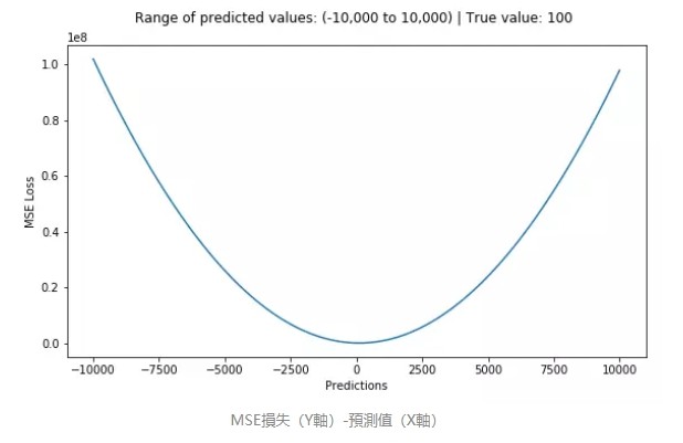
均方誤差 (MSE) 是最常用的回歸損失函數,計算方法是求預測值與真實值之間距離的平方和,公式如圖。
下圖是 MSE 函數的圖像,其中目標值是 100,預測值的範圍從 -10000 到 10000,Y 軸代表的 MSE 取值範圍是從 0 到正無窮,並且在預測值為 100 處達到最小。

-
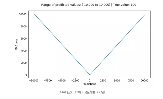
機器學習大神最常用的 5 個回歸損失函數,你知道幾個? | TechOrange
平均絕對誤差(MAE)是另一種用於回歸模型的損失函數。MAE 是目標值和預測值之差的絕對值之和。其只衡量了預測值誤差的平均模長,而不考慮方向,取值範圍也是從 0 到正無窮(如果考慮方向,則是殘差/誤差的總和——平均偏差(MBE))。
MSE 對誤差取了平方(令 e=真實值-預測值),因此若 e>1,則 MSE 會進一步增大誤差。如果數據中存在異常點,那麼 e 值就會很大,而 e²則會遠大於|e|。
因此,相對於使用 MAE 計算損失,使用 MSE 的模型會賦予異常點更大的權重。在第二個例子中,用 RMSE 計算損失的模型會以犧牲了其他樣本的誤差為代價,朝著減小異常點誤差的方向更新。然而這就會降低模型的整體性能。
如果訓練數據被異常點所污染,那麼 MAE 損失就更好用(比如,在訓練數據中存在大量錯誤的反例和正例標記,但是在測試集中沒有這個問題)。
直觀上可以這樣理解:如果我們最小化 MSE 來對所有的樣本點只給出一個預測值,那麼這個值一定是所有目標值的平均值。但如果是最小化 MAE,那麼這個值,則會是所有樣本點目標值的中位數。眾所周知,對異常值而言,中位數比均值更加魯棒,因此 MAE 對於異常值也比 MSE 更穩定。
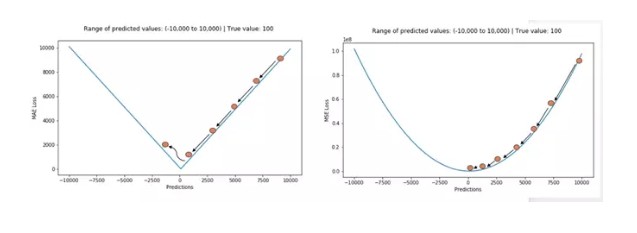
然而 MAE 存在一個嚴重的問題(特別是對於神經網絡):更新的梯度始終相同,也就是說,即使對於很小的損失值,梯度也很大。這樣不利於模型的學習。為了解決這個缺陷,我們可以使用變化的學習率,在損失接近最小值時降低學習率。
而 MSE 在這種情況下的表現就很好,即便使用固定的學習率也可以有效收斂。MSE 損失的梯度隨損失增大而增大,而損失趨於 0 時則會減小。這使得在訓練結束時,使用 MSE 模型的結果會更精確。

-
機器學習大神最常用的 5 個回歸損失函數,你知道幾個? | TechOrange
Huber 損失對數據中的異常點沒有平方誤差損失那麼敏感。它在 0 也可微分。本質上,Huber 損失是絕對誤差,只是在誤差很小時,就變為平方誤差。誤差降到多小時變為二次誤差由超參數 δ(delta)來控制。當 Huber 損失在 [0-δ,0+δ] 之間時,等價為 MSE,而在 [-∞,δ] 和 [δ,+∞] 時為 MAE。
這裡超參數 delta 的選擇非常重要,因為這決定了你對與異常點的定義。當殘差大於 delta,應當採用 L1(對較大的異常值不那麼敏感)來最小化,而殘差小於超參數,則用 L2 來最小化。
為何要使用 Huber 損失?
使用 MAE 訓練神經網絡最大的一個問題就是不變的大梯度,這可能導致在使用梯度下降快要結束時,錯過了最小點。而對於 MSE,梯度會隨著損失的減小而減小,使結果更加精確。
在這種情況下,Huber 損失就非常有用。它會由於梯度的減小而落在最小值附近。比起 MSE,它對異常點更加魯棒。因此,Huber 損失結合了 MSE 和 MAE 的優點。但是,Huber 損失的問題是我們可能需要不斷調整超參數 delta。

-
機器學習大神最常用的 5 個回歸損失函數,你知道幾個? | TechOrange
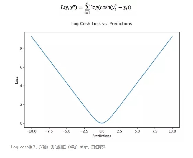
Log-cosh 是另一種應用於回歸問題中的,且比 L2 更平滑的的損失函數。它的計算方式是預測誤差的雙曲餘弦的對數。
優點:對於較小的 x,log(cosh(x)) 近似等於 (x^2)/2,對於較大的 x,近似等於 abs(x)-log(2)。這意味著’logcosh’ 基本類似於均方誤差,但不易受到異常點的影響。它具有 Huber 損失所有的優點,但不同於 Huber 損失的是,Log-cosh 二階處處可微。
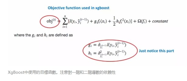
為什麼需要二階導數?許多機器學習模型如 XGBoost,就是採用牛頓法來尋找最優點。而牛頓法就需要求解二階導數(Hessian)。因此對於諸如 XGBoost 這類機器學習框架,損失函數的二階可微是很有必要的。
但 Log-cosh 損失也並非完美,其仍存在某些問題。比如誤差很大的話,一階梯度和 Hessian 會變成定值,這就導致 XGBoost 出現缺少分裂點的情況。
-
機器學習大神最常用的 5 個回歸損失函數,你知道幾個? | TechOrange
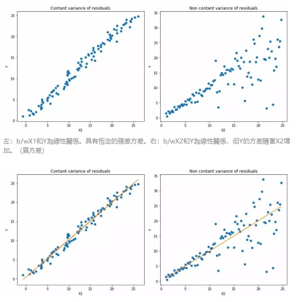
當我們更關注區間預測而不僅是點預測時,分位數損失函數就很有用。使用最小二乘回歸進行區間預測,基於的假設是殘差(y-y_hat)是獨立變量,且方差保持不變。
一旦違背了這條假設,那麼線性回歸模型就不成立。但是我們也不能因此就認為使用非線性函數或基於樹的模型更好,而放棄將線性回歸模型作為基線方法。這時,分位數損失和分位數回歸就派上用場了,因為即便對於具有變化方差或非正態分佈的殘差,基於分位數損失的回歸也能給出合理的預測區間。
下面讓我們看一個實際的例子,以便更好地理解基於分位數損失的回歸是如何對異方差數據起作用的。
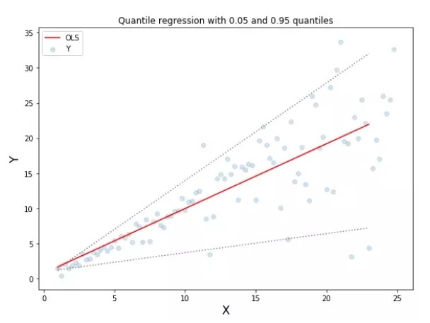
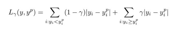
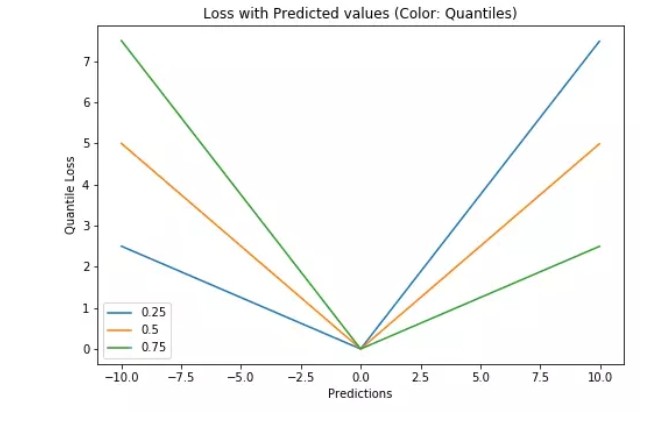
如何選取合適的分位值取決於我們對正誤差和反誤差的重視程度。損失函數通過分位值(γ)對高估和低估給予不同的懲罰。例如,當分位數損失函數 γ=0.25 時,對高估的懲罰更大,使得預測值略低於中值。
γ 是所需的分位數,其值介於 0 和 1 之間。
這個損失函數也可以在神經網絡或基於樹的模型中計算預測區間。以下是用 Sklearn 實現梯度提升樹回歸模型的示例。
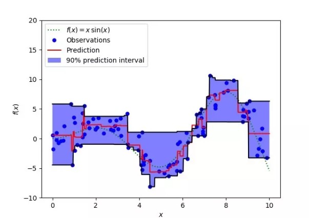
上圖表明:在 sklearn 庫的梯度提升回歸中使用分位數損失可以得到 90% 的預測區間。其中上限為 γ=0.95,下限為 γ=0.05。
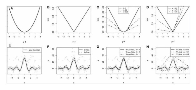
對比研究
為了證明上述所有損失函數的特點,讓我們來一起看一個對比研究。首先,我們建立了一個從 sinc(x)函數中採樣得到的數據集,並引入了兩項人為噪聲:高斯噪聲分量 ε〜N(0,σ2)和脈衝噪聲分量 ξ〜Bern(p)。
加入脈衝噪聲是為了說明模型的魯棒效果。以下是使用不同損失函數擬合 GBM 回歸器的結果。
連續損失函數:(A)MSE 損失函數;(B)MAE 損失函數;(C)Huber 損失函數;(D)分位數損失函數。將一個平滑的 GBM 擬合成有噪聲的 sinc(x)數據的示例:(E)原始 sinc(x)函數;(F)具有 MSE 和 MAE 損失的平滑 GBM;(G)具有 Huber 損失的平滑 GBM ,且δ={4,2,1};(H)具有分位數損失的平滑的 GBM,且α={0.5,0.1,0.9}。
仿真對比的一些觀察結果:
- MAE 損失模型的預測結果受脈衝噪聲的影響較小,而 MSE 損失函數的預測結果受此影響略有偏移。
- Huber 損失模型預測結果對所選超參數不敏感。
- 分位數損失模型在合適的置信水平下能給出很好的估計。