Big O notation is a way to describe the performance of an algorithm by analysing its time or space complexity as a function of input size. It provides an upper bound on the growth rate of an algorithm's resource consumption (time or space), which helps us understand how the algorithm's performance will scale as the input size increases.
The term "Big O" comes from the fact that it represents the "order" of the function describing the relationship between the input size and the resource consumption. In Big O notation, we only consider the highest-degree term of the function, as this term dominates the growth rate when the input size becomes large. We also ignore any constant factors, since they do not affect the growth rate.
Here are some common examples of Big O notation and their corresponding functions:
- O(1): Constant time complexity. The algorithm's performance does not depend on the input size. Examples include array element access or simple arithmetic operations.
- O(log n): Logarithmic time complexity. The algorithm's performance grows logarithmically with the input size. Binary search is an example of an algorithm with O(log n) complexity.
- O(n): Linear time complexity. The algorithm's performance grows linearly with the input size. Examples include searching for an element in an unsorted array or simple iterations through a list.
- O(n log n): Linearithmic time complexity. The algorithm's performance grows linearly and logarithmically with the input size. Many efficient sorting algorithms, such as merge sort and quicksort, have O(n log n) complexity.
- O(n^2): Quadratic time complexity. The algorithm's performance grows quadratically with the input size. Nested loops with simple operations, such as insertion sort or bubble sort, often have O(n^2) complexity.
- O(n^3): Cubic time complexity. The algorithm's performance grows cubically with the input size. Examples include certain matrix multiplication algorithms.
- O(2^n): Exponential time complexity. The algorithm's performance grows exponentially with the input size. Examples include some recursive algorithms like the naive implementation of Fibonacci sequence calculation.
- O(n!): Factorial time complexity. The algorithm's performance grows factorially with the input size. Examples include some brute-force algorithms for solving the traveling salesman problem.
Big O notation helps us compare different algorithms' performance and choose the most appropriate one for a particular problem or situation. It is important to note that Big O notation only provides an asymptotic upper bound and does not guarantee the actual performance of an algorithm in practice. However, it serves as a useful tool for understanding how algorithms scale with increasing input size.
A stack is a collection of elements, with two main operations: pushing an element onto the stack, and popping it off. The elements are stored in a last-in, first-out (LIFO) order.
A stack is a linear data structure that follows the LIFO (Last-In-First-Out) principle and only has one end. A stack is an abstract data type that serves as a collection of elements, with two principal operations:
- push, which adds an element to the collection, and
- pop, which removes the most recently added element that was not yet removed.
The order in which elements come off a stack gives rise to its alternative name, LIFO (last in, first out). Additionally, a peek operation may give access to the top without modifying the stack. The name "stack" for this type of structure comes from the analogy to a set of physical items stacked on top of each other, which makes it easy to take an item off the top of the stack, while getting to an item deeper in the stack may require taking off multiple other items first.

class Stack<T> {
  _store: T[] = [];
  push(val: T) {
    this._store.push(val);
  }
  pop(): T | undefined {
    return this._store.pop();
  }
}A queue is a data structure that stores elements in a linear fashion, where we can add elements to the end (enqueue) and remove elements from the front (dequeue), like a real-life queue.
A queue is a particular kind of abstract data type or collection in which the entities in the collection are kept in order and the principle (or only) operations on the collection are the addition of entities to the rear terminal position, known as enqueue, and removal of entities from the front terminal position, known as dequeue. This makes the queue a First-In-First-Out (FIFO) data structure. In a FIFO data structure, the first element added to the queue will be the first one to be removed.
This is equivalent to the requirement that once a new element is added, all elements that were added before have to be removed before the new element can be removed. Often a peek or front operation is also entered, returning the value of the front element without dequeuing it. A queue is an example of a linear data structure, or more abstractly a sequential collection.

class Queue<T> {
  _store: T[] = [];
  push(val: T) {
    this._store.push(val);
  }
  pop(): T | undefined {
    return this._store.shift();
  }
}A linked list is a collection of “nodes” connected together via links. These nodes consist of the data to be stored and a pointer to the address of the next node within the linked list. In the case of arrays, the size is limited to the definition, but in linked lists, there is no defined size. Any amount of data can be stored in it and can be deleted from it.
- Singly Linked List − The nodes only point to the address of the next node in the list.
- Doubly Linked List − The nodes point to the addresses of both previous and next nodes.
- Circular Linked List − The last node in the list will point to the first node in the list. It can either be singly linked or doubly linked.
A singly linked list is a data structure that consists of elements called nodes, where each node points to the next node in the sequence. It is called "singly" because each node has a single reference to the next node. It can only traverse in one direction.
A doubly linked list is similar to a singly linked list, but each node has two references: one to the next node and another to the previous node. This allows traversing the list in both directions.
A hash table, also known as a hash map, is a data structure that allows you to store and retrieve values based on their associated keys. It provides an efficient way to perform lookups, insertions, and deletions in near-constant time. Hash tables achieve this efficiency by using a hashing function to map keys to indices in an underlying array, known as the "buckets" array.
Here's a high-level overview of how a hash table works:
- Hashing function: The hash table uses a hash function to convert the input key into an integer value, known as the hash code. The hash function should have a few essential properties: it should be deterministic (i.e., always return the same hash code for the same key), it should distribute keys uniformly across the array to avoid clustering, and it should be fast to compute.
- Bucket index computation: The hash code is then used to calculate an index in the underlying array where the key-value pair should be stored. This is often done by using the modulo operator, which takes the remainder of the division between the hash code and the array size (i.e.,
index = hashCode % arraySize). This ensures that the calculated index falls within the bounds of the array. - Handling collisions: Since the array has a finite size, it is possible for two different keys to have the same hash code, or for their hash codes to map to the same index after the modulo operation. This situation is called a collision. There are several techniques to handle collisions, such as separate chaining (using a linked list to store all the key-value pairs with the same index) or open addressing (looking for the next available slot in the array using a process called probing).
- Resizing: As the hash table becomes more full, the likelihood of collisions increases, which can negatively impact performance. To maintain efficiency, it is common to resize the hash table by increasing the size of the underlying array and rehashing all the existing keys.
Overall, hash tables are a powerful data structure for storing and retrieving data quickly. They have an average-case time complexity of O(1) for insertion, deletion, and lookup operations, making them suitable for various applications, such as caches, symbol tables, or dictionaries. However, their worst-case time complexity can be O(n) if there are many collisions or the hash table is poorly implemented.


A tree is a hierarchical data structure that consists of nodes connected by edges. It is a non-linear data structure, unlike arrays or linked lists, and is used to represent relationships between objects in a hierarchical manner. Each node in a tree can have zero, one, or multiple child nodes, and a single parent node, except for the root node, which has no parent.
Here are some key features and terminology associated with tree data structures:
- Root: The topmost node in the tree, which has no parent. There is only one root node in a tree.
- Edges: The connections between nodes in the tree. Each edge represents a relationship between two nodes: a parent and a child.
- Children: Nodes that have a parent node. These nodes are one level below their parent node in the hierarchy.
- Parent: A node that has one or more child nodes connected to it.
- Leaf: A node with no children. Leaf nodes are the "endpoints" of the tree.
- Siblings: Nodes that share the same parent.
- Depth: The number of edges in the path from the root node to a particular node. The root node has a depth of 0.
- Height: The maximum depth of any node in the tree.
- Internal node: A node that has at least one child (i.e., not a leaf node).
- Degree: The number of children a node has. The degree of a tree is the maximum degree of any node in the tree.
Trees are used in many computer science applications, including file systems, databases, parsing, and artificial intelligence. There are several types of trees, such as binary trees (where each node has at most two children), balanced trees (e.g., AVL trees or red-black trees), and B-trees (used in databases and file systems).
Trees are an efficient way to represent hierarchical relationships, search and organise data, and perform various operations, such as insertion, deletion, and traversal. The time complexity of operations on trees depends on the type of tree and its height. For balanced trees, most operations have a time complexity of O(log n), where n is the number of nodes in the tree.

A binary tree is a hierarchical data structure in which each node has at most two children, referred to as the left child and the right child. It is a type of tree data structure that is widely used in computer science due to its simplicity and versatility.
Binary trees are composed of nodes, which contain a value and two pointers (or references) to their left and right children. The topmost node in the tree is called the root, which has no parent. Nodes with the same parent are called siblings. A node with no children is called a leaf node.
Some key concepts associated with binary trees are:
- Root: The topmost node in the tree, which has no parent.
- Parent: A node that has one or more child nodes connected to it.
- Child: A node that has a parent node.
- Siblings: Nodes that share the same parent.
- Leaf: A node with no children.
- Depth: The number of edges in the path from the root node to a particular node. The root node has a depth of 0.
- Height: The maximum depth of any node in the tree.
Binary trees can be used in various applications, such as expression parsing, syntax analysis in compilers, data compression (e.g., Huffman encoding), and decision trees in machine learning. There are several types of binary trees with specific properties, such as:
- Full binary tree: Every level of the tree is completely filled, except possibly for the last level, which is filled from left to right.
- Complete binary tree: Every level is completely filled, and all nodes in the last level are as far left as possible.
- Perfect binary tree: Every level is completely filled, including the last level.
- Skewed binary tree: A binary tree where all nodes have only one child, either left or right. This makes the tree resemble a linked list.
Binary trees can be traversed in various ways, such as pre-order (root, left, right), in-order (left, root, right), and post-order (left, right, root) traversal. The time complexity of traversing a binary tree is O(n), where n is the number of nodes in the tree, as each node is visited once.
A Binary Search Tree (BST) is a tree data structure in which each node has at most two children, called left and right child. The key property of a Binary Search Tree is that the value of a node's left child is less than or equal to the value of the node itself, and the value of its right child is greater than or equal to the node's value. This ordering property ensures that a binary search can be run efficiently on the BST.
A binary search trees (BST), sometimes called ordered or sorted binary trees, are a particular type of container: data structures that store "items" (such as numbers, names etc.) in memory. They allow fast lookup, addition and removal of items, and can be used to implement either dynamic sets of items, or lookup tables that allow finding an item by its key (e.g., finding the phone number of a person by name).
Binary search trees keep their keys in sorted order, so that lookup and other operations can use the principle of binary search: when looking for a key in a tree (or a place to insert a new key), they traverse the tree from root to leaf, making comparisons to keys stored in the nodes of the tree and deciding, on the basis of the comparison, to continue searching in the left or right subtrees.
On average, this means that each comparison allows the operations to skip about half of the tree, so that each lookup, insertion or deletion takes time proportional to the logarithm of the number of items stored in the tree. This is much better than the linear time required to find items by key in an (unsorted) array, but slower than the corresponding operations on hash tables.
A Binary Search Tree provides an efficient way to store and retrieve data in a sorted order. Its average-case time complexity for search, insertion, and deletion operations is O(log n), where n is the number of nodes in the tree. However, in the worst case, when the tree becomes unbalanced and degenerates into a linked list, the time complexity can degrade to O(n). To avoid this, there are self-balancing Binary Search Trees, such as AVL trees and Red-Black trees, which maintain a balanced structure to ensure optimal performance.
| Access | Search | Insertion | Deletion |
|---|---|---|---|
O(log(n)) |
O(log(n)) |
O(log(n)) |
O(log(n)) |
O(n)

A binary tree and a binary search tree are both hierarchical data structures composed of nodes, with each node having at most two children (left and right). However, they differ in terms of the properties and constraints on the organisation of the nodes.
Binary Tree: A binary tree is a general tree data structure where each node can have a maximum of two children. There is no specific ordering or relationship between the nodes, which means that the values in the nodes can be arranged in any way. Binary trees are used in a variety of applications, such as expression trees, Huffman encoding, and decision trees in machine learning.
Binary Search Tree (BST): A binary search tree is a more specialised version of a binary tree with a specific ordering property. In a binary search tree, for every node:
- All the nodes in its left subtree have values less than the node's value.
- All the nodes in its right subtree have values greater than the node's value.
This ordering property allows binary search trees to support efficient search, insertion, and deletion operations. The time complexity for these operations in a balanced BST is O(log n), where n is the number of nodes. However, in the worst case (e.g., when the BST is completely unbalanced and becomes a linked list), the time complexity can be O(n). To maintain efficiency, self-balancing binary search trees like AVL trees or red-black trees are often used.
In summary, a binary tree is a more general data structure with no specific ordering between the nodes, while a binary search tree is a specialised binary tree with a strict ordering property that enables efficient search, insertion, and deletion operations.
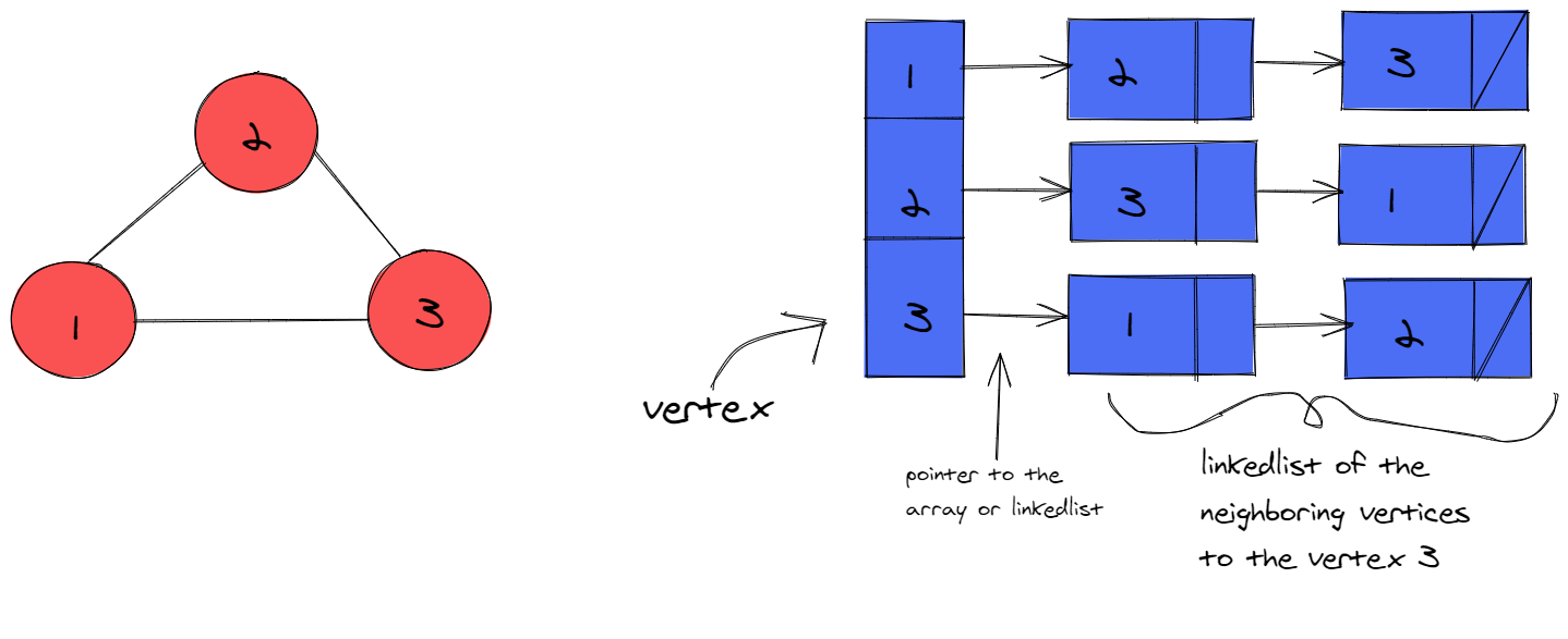
A graph is a data structure that represents the relationship between different objects, often called nodes or vertices. Imagine a group of friends where each person is a node, and their friendships are the connections (also called edges) between them. A graph helps us visualise and work with such relationships.
There are two main types of graphs:
- Undirected Graph: The connections between nodes don't have a direction, meaning if node A is connected to node B, then node B is also connected to node A. An example would be Facebook friendships, where if you are friends with someone, they are also friends with you.
- Directed Graph: The connections between nodes have a direction. If node A is connected to node B, it doesn't mean node B is connected to node A. An example would be Twitter followers, where if you follow someone, they don't necessarily follow you back.
Graphs can also be categorised based on the presence of edge weights:
- Unweighted Graph: The edges in the graph do not have any associated weight or cost. All edges are considered to have the same weight.
- Weighted Graph: The edges in the graph have an associated weight or cost, which represents the strength or cost of the relationship between the connected vertices. Weighted graphs are commonly used in problems involving pathfinding or shortest-path algorithms.
Graphs can be represented in memory using various data structures, such as:
- Adjacency Matrix: A two-dimensional matrix (usually a square matrix) is used to represent the graph. The element at the ith row and jth column of the matrix is set to 1 (or the edge weight) if there is an edge between vertex i and vertex j, and 0 otherwise. This representation is space inefficient for sparse graphs (graphs with few edges), as it requires O(V^2) space, where V is the number of vertices.

- Adjacency List: An array or list of lists is used to represent the graph, where each element in the array corresponds to a vertex, and the associated list contains the neighbours of that vertex. This representation is more space-efficient for sparse graphs, as it requires O(V + E) space, where E is the number of edges.
Graphs can be traversed using various algorithms, such as Depth-First Search (DFS) or Breadth-First Search (BFS), to explore the relationships between vertices, find paths, or solve other graph-related problems. The time complexity of these traversal algorithms is generally O(V + E), where V is the number of vertices and E is the number of edges.


const graph: Map<string, string[]> = new Map<string, string[]>([
  ['A', ['B', 'C']],
  ['B', ['A', 'D', 'E']],
  ['C', ['A', 'E']],
  ['D', ['B']],
  ['E', ['B', 'C']],
]);
Binary Search is an efficient algorithm for finding a specific element in a sorted array. It works by repeatedly dividing the array into two halves - one with elements smaller than the target, and the other with elements larger than the target. It then narrows down the search by only considering the half that may contain the target element. This process continues until the desired element is found or until the search space becomes empty.
The time complexity of the binary search algorithm is O(log n). The best-case time complexity would be O(1) when the central index would directly match the desired value.
NOTE: Binary Search only works with sorted arrays, so it's essential to sort the array using Quick Sort or any other sorting algorithm before performing the search.
Quick Sort is a widely used, efficient sorting algorithm that works based on the "divide and conquer" approach. It sorts a list or an array of elements by selecting a "pivot" element and then partitioning the elements into two smaller groups:
- Elements less than or equal to the pivot
- Elements greater than the pivot
Quick Sort then recursively applies the same process to the two smaller groups until the entire list is sorted.
Here's a high-level overview of the Quick Sort algorithm:
- Choose a pivot element from the list. The choice of pivot can impact the algorithm's performance; common strategies include selecting the first, last, middle, or a random element.
- Partition the list into two groups based on the pivot: one group with elements less than or equal to the pivot and another group with elements greater than the pivot.
- Recursively apply Quick Sort to both groups.
- Combine the two groups (now sorted) with the pivot in between.
Let's go through an example to better understand the process. Suppose we have the following list of numbers:
8, 3, 5, 1, 7, 4, 6
We'll choose the first element as the pivot (8). After partitioning the list based on the pivot, we get:
[3, 5, 1, 7, 4, 6] and [8]
Now, we apply Quick Sort recursively to both groups:
[3, 5, 1, 7, 4, 6] -> [1, 3, 4, 5, 6, 7][8] -> [8]
Finally, we combine the two sorted groups and the pivot:
[1, 3, 4, 5, 6, 7, 8]
The list is now sorted. Note that the choice of pivot and the order of elements in the original list can impact the algorithm's performance. In the best and average cases, Quick Sort has a time complexity of O(n log n), where n is the number of elements. However, in the worst case (already sorted list with a poorly chosen pivot), the time complexity can be O(n^2).
Merge Sort is an efficient sorting algorithm that uses the "divide and conquer" strategy. It works by dividing a list or an array of elements into smaller parts, sorting them independently, and then merging the sorted parts to create a fully sorted list.
Here's a high-level overview of the Merge Sort algorithm:
- Divide the list into two equal halves.
- Recursively apply Merge Sort to both halves.
- Merge the two sorted halves to create a fully sorted list.
The key to the Merge Sort algorithm is the "merge" step, which combines two sorted lists into a single sorted list. This step is performed in linear time, meaning it takes O(n) time, where n is the total number of elements in the two lists.
Let's go through an example to better understand the process. Suppose we have the following list of numbers:
5, 1, 8, 3, 6, 4, 7
First, we divide the list into two halves:
[5, 1, 8] and [3, 6, 4, 7]
Now, we recursively apply Merge Sort to both halves:
[5, 1, 8] -> [1, 5, 8][3, 6, 4, 7] -> [3, 4, 6, 7]
Finally, we merge the two sorted halves:
[1, 5, 8] and [3, 4, 6, 7] -> [1, 3, 4, 5, 6, 7, 8]
The list is now sorted. Merge Sort has a time complexity of O(n log n) in the best, average, and worst cases, where n is the number of elements. This makes it a reliable and efficient sorting algorithm for various applications. However, it often requires additional space for the merging process, which can be a disadvantage compared to some in-place sorting algorithms like Quick Sort.
Breadth First Search (BFS) is a graph traversal algorithm that explores all the nodes of a graph in a layer-by-layer manner. Imagine you're trying to explore a maze, and you want to visit all the rooms. BFS allows you to visit all the rooms in the order of their distance from your starting point.
Here's how the BFS algorithm works:
- Start at the initial node (or the starting point).
- Visit all the neighbours of the starting node.
- For each neighbour, visit all of its neighbours that haven't been visited yet.
- Repeat step 3 until all the nodes in the graph have been visited.
During the traversal process, BFS uses a queue data structure to keep track of the nodes to visit. The queue ensures that we visit nodes in the order they are discovered.
Let's use the following graph as an example:
A -- B -- D
|    |
C -- E
If we start at node A and apply the BFS algorithm, the traversal order would be: A, B, C, D, E.
Here's a step-by-step explanation of the process:
- Start at node A, mark it as visited, and add its neighbours (B and C) to the queue.
- Dequeue the first node in the queue (B), mark it as visited, and add its unvisited neighbours (D and E) to the queue.
- Dequeue the next node in the queue (C), mark it as visited, and add its unvisited neighbours (none) to the queue.
- Dequeue the next node in the queue (D), mark it as visited, and add its unvisited neighbours (none) to the queue.
- Dequeue the last node in the queue (E), mark it as visited, and add its unvisited neighbours (none) to the queue.
At this point, the queue is empty, and we've visited all the nodes in the graph.
Depth First Search (DFS) is a graph traversal algorithm that explores the nodes of a graph by visiting a node and then recursively exploring its neighbours as deep as possible before backtracking. In other words, it goes as deep as it can along a path before going back to explore other paths.
Imagine you're exploring a treehouse with multiple levels and branches. DFS would be like climbing all the way to the top of one branch, then climbing down and moving to the next branch, and so on.
Here's how the DFS algorithm works:
- Start at the initial node (or the starting point).
- Visit the node and mark it as visited.
- For each neighbour of the current node that hasn't been visited, recursively apply the DFS algorithm.
- If there are no more unvisited neighbours, backtrack (return) to the previous node and continue the process.
Let's use the following graph as an example:
A -- B -- D
|    |
C -- E
If we start at node A and apply the DFS algorithm, one possible traversal order would be: A, B, D, E, C.
Here's a step-by-step explanation of the process:
- Start at node A, mark it as visited, and recursively apply the DFS algorithm on its first neighbour (B).
- Visit node B, mark it as visited, and recursively apply the DFS algorithm on its first neighbour (D).
- Visit node D, mark it as visited, and since it has no unvisited neighbours, backtrack to node B.
- At node B, move to the next unvisited neighbour (E), mark it as visited, and recursively apply the DFS algorithm on it.
- Visit node E, mark it as visited, and recursively apply the DFS algorithm on its only unvisited neighbour (C).
- Visit node C, mark it as visited, and since it has no unvisited neighbours, backtrack to E, then B, then A.
At this point, we've visited all the nodes in the graph using the DFS algorithm. Note that the traversal order might be different depending on the order in which neighbours are visited.
The Fibonacci sequence is a series of numbers where each number is the sum of the two preceding ones, usually starting with 0 and 1. So, the sequence goes: 0, 1, 1, 2, 3, 5, 8, 13, and so on.
Memoization is a technique where we store the results of expensive function calls and return the cached result when the same inputs occur again. This helps us save time and resources, as we don't need to compute the result every time the function is called with the same input. So, when you call the fibonacci function with the same input multiple times, it will return the result from the cache instead of recalculating it.
A Palindrome is a word, phrase, number, or other sequence of characters which reads the same backward or forward. A Palindrome is a word, phrase, number, or other sequence of characters which reads the same backward or forward.
function isPalindrome(str:string) {
  return str.split('').reverse().join('') === str;
}JavaScript string doesn't have a reverse method. But you can just use the Array.prototype.reverse method.
function reverse(str:string) {
  return str.split('').reverse().join('');
}