- Problem Statement
- Similarity Learning Tasks
- Evaluation Metrics
- Establishing Baselines
- About Datasets and Models
- The journey
- Benchmarked Models
- Notes on Finetuning Models
- Thoughts on Deep Learning Models
- Conclusion
- Future Work
The task of Similarity Learning is a task of learning similarities or disimilarites between sentences/paragraphs. The core idea is to find some sort of vector representation for a sentence/document/paragraph. This vector representation can then be used to compare a given sentence with other sentences. For example
Let's say we want to compare the sentences: "Hello World", "Hi there friend" and "Bye bye".
We have to develop a function, similarity_fn such that
similarity_fn("Hello there", "Hi there friend") > similarity_fn("Hello there friend", "Bye Bye")
similarity_fn("Hello there", "Hi there friend") = 0.9
similarity_fn("Hello there friend", "Bye Bye") = 0.1
As such, Similarity Learning does not require Neural Networks (tf-idf and other such sentence representations can work as well). However, with the recent domination of Deep Learning in NLP, newer models have been performing the best on Similarity Learning tasks.
The idea of finding similarities can be used in the following ways :
1. Regresssion Similarity Learning: given document1 and document2 we need a similiarity measure as a float value.
2. Classification Similarity Learning: given document1 and document2 we need to classify them as similar or disimilar
3. Ranking Similarity Learning: given document, similar-document and disimilar-document, we want to learn a similarity_function such that similarity_function(document, similar-document) > similarity_function(document, disimilar-document)
Usually, the similarity can be measures like:
- A vector representation is calculated for the two documents and the cosine similarity between them is their similarity score
- The two documents are made to interact in several different ways (neural attention, matrix multiplication, LSTMs) and a softmax probablity is calculated of them being similar or dissimilar. Example:
[0.2, 0.8] -> [probablity of being dissimilar, probablity of being similar]
1. Question Answering/Information Retrieval
Given a question and a number of candidate answers, we want to rank the answers based on their likelihood of being the answer to the question.
Example:
Q: When was Gandhi born?
A1: Gandhi was a freedom fighter
A2: He was born 2 October, 1989
A3: He was a freedom fighter
The answer selected by the model is
argmax_on_A(simialrity_fn(Q, A1), simialrity_fn(Q, A2), simialrity_fn(Q, A3)) = A2
Conversation/Respone Selection is similar to Question Answering, for a given Question Q, we want to select the most appropriate response from a pool of responses (A1, A2, A3, ...)
Example datasets: WikiQA
2. Textual Entailment
Given a text and a hypothesis, the model must make a judgement to classify the text
Example from SICK:
| The young boys are playing outdoors and the man is smiling nearby | There is no boy playing outdoors and there is no man smiling | CONTRADICTION |
| A skilled person is riding a bicycle on one wheel | A person is riding the bicycle on one wheel | ENTAILMENT |
| The kids are playing outdoors near a man with a smile | A group of kids is playing in a yard and an old man is standing in the background | NEUTRAL |
3. Duplicate Document Detection/Paraphrase Detection
Given 2 docs/sentences/questions we want to predict the probablity of the two questions being duplicate
Example:
- "What is the full form of AWS" -- "What does AWS stand for?" --> Duplicate
- "What is one plus one?" -- "Who is president?" --> Not Duplicate
Example Dataset: Quora Duplicate Question Dataset
4. Span Selection:
Given a context passage and a question, we have to find the span of words in the passage which answers the question.
Example:
passage: "Bob went to the doctor. He wasn't feeling too good"
question: "Who went to the doctor"
span: "*Bob* went to the doctor. He wasn't feeling too good"
Example Dataset: SQUAD
While some similarity functions have simple metrics(Accuracy, Precision), it can get a bit complicated/different for others.
Duplicate Question/Paraphrase Detection and Textual Entailment use Accuracy.
Since it is easy to say that an answer is either correct or incorrect. Accuracy is simply the ratio of correct answers to the total number of questions.
Span Selection uses Exact Match and F1 score
How many times did the model predict the correct span?
(A full list of datasets and metrics can be found here)
It gets a bit tricky when you come to evaluate Question Answering systems. The reason for this is: The results given by these systems is usually in an ordereing of the candidate documents.
For a query Q1 and set of candidate answers (very-relevant-answer, slightly-relevant-answer, irrelevant-answer)
The evaluation metric should score the ordering of
(1: very-relevant-answer, 2: slightly-relevant-answer, 3:irrelevant-answer) > (1: slightly-relevant-answer, 2: very-relevant-answer, 3:irrelevant-answer) > (1: irrelevant-answer, 2: slightly-relevant-answer, 3:irrelevant-answer)
Basically, the metric should give a higher score to an ordering where the more relevant documents come first and less relevant documents come later.
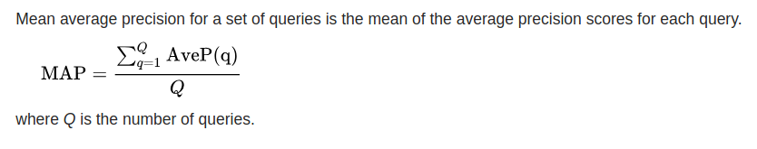
The metric commonly used for this are Mean Average Precision(MAP), Mean Reciprocal Rank(MRR) and Normalized Discounted Cumulative Gain(nDCG).
You can read more here It is a measure to be calculated over a full dataset. A dataset like WikiQA, will have a setup like:
q_1, (d1, d2, d3)
q_2, (d4, d5)
q_3, (d6, d7, d8, d9, d10)
.
.
.
we find the average precision for every q_i and then take the mean over all the qs
Mean (Over all the queries) Average Precision(Over all the docs for a query)
Some psuedo code to describe the idea:
num_queries = len(queries)
precision = 0
for q, candidate_docs in zip(queries, docs):
    precision += average_precision(q, candidate_docs)
mean_average_precision = precision / num_queries
I will solve an example here:
Model predictions: (q1-d1, 0.2), (q1-d2, 0.7) , (q1-d3, 0.3)
Ground Truth     : (q1-d1, 1),   (q1-d2, 1) ,     (q1-d3, 0)
We will sort our predictions based on our similarity score (Since our ordering/ranking is in that order)
(d2, 0.7, 1), (d3, 0.3, 0), (d1, 0.2, 1)


Average Precision = (Sum (Precision@k * relevance@k) for k=1 to n) / Number of Relevant documents
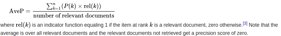
where
n : the number of candidate docs
relevance@k : 1 if the kth doc is relevant, 0 if not
Precision@k : precision till the kth cut off where precision is : (number of retrieved relevant docs / total retrieved docs)
So, Average Precision = (1/1 + 0 + 2/3)/2 = 0.83
Here's how:
At this point, we can discard our score (since we've already used it for ordering)
(d2, 1) (d3, 0) (d1, 1)
Number of Relevant Documents is (1 + 0 + 1) = 2
Precision at 1: We only look at (d2, 1)
p@1 = (number of retrieved relevant@1/total number of retrieved docs@1) * relevance@1
    = (1 / 1) * 1
    = 1
Precision at 2: We only look at (d2, 1) (d3, 0)
p@2 = (number of retrieved relevant@2/total number of retrieved docs@2) * relevance@2
    = (1 / 2) * 0
    = 0
Precision at 3: We only look at (d2, 1) (d3, 0) (d1, 1)
p@3 = (number of retrieved relevant@3/total number of retrieved docs@3) * relevance@3
    = (2 / 3) * 1
    = 2/3
Therefore, Average Precision for q1
								= (Precision@1 + Precision@2 + Precision@3) / Number of Relevant Documents
                                = (1 + 0 + 2/3) / 2
                                = 0.83
To get Mean Average Precision, we calculate Average Precision for all qs in it and average it/take the mean.
This Wikipedia Article is a great source for understanding NDCG. First, let's understand Discounted Cumulative Gain.
The premise of DCG is that highly relevant documents appearing lower in a search result list should be penalized as the graded relevance value is reduced logarithmically proportional to the position of the result.
DCG@P = Sum for i=1 to P (relevance_score(i) / log2(i + 1))
Let's take the previous example:
(d2, 0.7, 1), (d3, 0.3, 0), (d1, 0.2, 1)
DCG@3 = 0.7/log2(1 + 1) + 0.3/log2(1 + 2) + 0.2/log2(1 + 3)
As can be seen, if a high score is given
For getting the Normalized Discounted:
Since result set may vary in size among different queries or systems, to compare performances the normalised version of DCG uses an ideal DCG. To this end, it sorts documents of a result list by relevance, producing an ideal DCG at position p ( {\displaystyle IDCG_{p}} IDCG_p), which normalizes the score:
nDCG = DCG / IDCG
Use MAP when you a candidate document is either relevant or not relevant (1 or 0)
Use nDCG when you have a range of values for relevance. For example, when documents have relevance (d1 : 1, d2: 2, d3: 3)
For a more detailed idea, refer to this issue on the MatchZoo repo.
As per @bwanglzu
@aneesh-joshi I'd say it can be evaluated with nDCG, but not meaningful or representative. For binary retrieval problem (say the labels are 0 or 1 indicates relevant or not), we use P, AP, MAP etc. For non-binary retrieval problem (say the labels are real numbers greater equal than 0 indicates the "relatedness"]), we use nDCG. In this situation, clearly, mAP@k is a better metric than nDCG@k. In some cases for non-binary retrieval problem, we use both nDCG & mAP such as microsoft learning to rank challenge link.
While the idea of the metric seems easy, there are varying implementations of it which can be found below in the section "MatchZoo Baselines". Ideally, the most trusted metric implementations should be the one provided by TREC and I would imagine that's what people use when publishing results.
The TextRetrievalConference(TREC) is an ongoing series of workshops focusing on a list of different information retrieval (IR) research areas, or tracks. They provide a standard method of evaluating QA systems called trec_eval. It's a C binary whose code can be found here
Please refer to this blog to get a complete understanding of trec
Here's the short version:
As the above tutorial link will tell, you will have to download the TREC evaluation code from here
run make in the folder and it will produce the trec_eval binary.
The binary requires 2 inputs:
- qrels: It is the query relevance file which will hold the correct answers.
- pred file: It is the predicition file which will have the predictions made by your model
It can be run like:
$ ./trec_eval qrels pred
The above will provide some standard metrics. You can also specify metrics on your own like:
$ ./trec_eval -m map -m ndcg_cut.1,3,5,10,20 qrels pred
The above will provide MAP value and nDCG at cutoffs of 1, 3, 5, 10 and 20
The qrels format is:
Format
------
<query_id>\t<0>\t<document_id>\t<relevance>

Note: parameter <0> is ignored by the model

Example
-------
Q1  0   D1-0    0
Q1  0   D1-1    0
Q1  0   D1-2    0
Q1  0   D1-3    1
Q1  0   D1-4    0
Q16 0   D16-0   1
Q16 0   D16-1   0
Q16 0   D16-2   0
Q16 0   D16-3   0
Q16 0   D16-4   0
The model's prediction, pred should be like:
Format
------
<query_id>\t<Q0>\t<document_id>\t<rank>\t<model_score>\t<STANDARD>

Note: parameters <Q0>, <rank> and <STANDARD> are ignored by the model and can be kept as anything
I have chose 99 as the rank. It has no meaning.

Example
-------
Q1  Q0  D1-0    99  0.64426434  STANDARD
Q1  Q0  D1-1    99  0.26972288  STANDARD
Q1  Q0  D1-2    99  0.6259719   STANDARD
Q1  Q0  D1-3    99  0.8891963   STANDARD
Q1  Q0  D1-4    99  1.7347554   STANDARD
Q16 Q0  D16-0   99  1.1078827   STANDARD
Q16 Q0  D16-1   99  0.22940424  STANDARD
Q16 Q0  D16-2   99  1.7198141   STANDARD
Q16 Q0  D16-3   99  1.7576259   STANDARD
Q16 Q0  D16-4   99  1.548423    STANDARD
In our journey of developing a similarity learning model, we first decided to use the WikiQA dataset since it is a well studied and common baseline used in many papers like SeqMatchSeq, BiMPM and QA-Transfer.
To understand the level of improvement we could make, we set up a baseline using word2vec. We use the average of word vectors in a sentence to get the vector for a sentence/document.
"Hello World" -> (vec("Hello") + vec("World"))/2
When 2 documents are to be compared for similarity/relevance, we take the Cosine Similarity between their vectors as their similarity. (300 dimensional vectors were seen to perform the best, so we chose them.)
The w2v 300 dim MAP score on the full set(100%) of WikiQA is 0.59
train split(80%) of WikiQA is 0.57
test split(20%) of WikiQA is 0.62
dev split(10%) of WikiQA is 0.62
I had found a repo called MatchZoo which had almost 10 different Similarity Learning models developed and benchmarked. According to their benchmarks, their best model performed around 0.65 MAP on WikiQA.
I tried to reproduce their results using their scripts but found that the scores weren't keeping up with what they advertised. I raised an issue. (There was a similar issue before mine as well.) They went about fixing it. I was later able to reproduce their results (by reverting to a point earlier in the commit history) but there was now a lack of trust in their results. I sought out to write my own script in order to make my evaluation independent of theirs. The problem was that they had their own way of representing words and other such internal functions. Luckily, they were dumping their results in the TREC format. I was able to scrape that and evaluate it using this script.
I developed a table with my baselines as below:

Note: the values are different from the established baseline because there is some discrepancy on how MAP should be calculated. I initially used my implementation of it for the table. Later, I moved to that provided by trec. This is how I implement it:
def mapk(Y_true, Y_pred):
    """Calculates Mean Average Precision(MAP) for a given set of Y_true, Y_pred

    Note: Currently doesn't support mapping at k. Couldn't use only map as it's a
    reserved word

    Parameters
    ----------
    Y_true : numpy array or list of ints either 1 or 0
        Contains the true, ground truth values of the relevance between a query and document
    Y_pred : numpy array or list of floats
        Contains the predicted similarity score between a query and document

    Examples
    --------
    >>> Y_true = [[0, 1, 0, 1], [0, 0, 0, 0, 1, 0], [0, 1, 0]]
    >>> Y_pred = [[0.1, 0.2, -0.01, 0.4], [0.12, -0.43, 0.2, 0.1, 0.99, 0.7], [0.5, 0.63, 0.92]]
    >>> print(mapk(Y_true, Y_pred))
    0.75
    """

    aps = []
    n_skipped = 0
    for y_true, y_pred in zip(Y_true, Y_pred):
        # skip datapoints where there is no solution
        if np.sum(y_true) < 1:
            n_skipped += 1
            continue

        pred_sorted = sorted(zip(y_true, y_pred), key=lambda x: x[1], reverse=True)
        avg = 0
        n_relevant = 0

        for i, val in enumerate(pred_sorted):
            if val[0] == 1:
                avg += 1. / (i + 1.)
                n_relevant += 1

        if n_relevant != 0:
            ap = avg / n_relevant
            aps.append(ap)
    return np.mean(np.array(aps))
This is how it's implemented in MatchZoo:
def map(y_true, y_pred, rel_threshold=0):
    s = 0.
    y_true = _to_list(np.squeeze(y_true).tolist())
    y_pred = _to_list(np.squeeze(y_pred).tolist())
    c = list(zip(y_true, y_pred))
    random.shuffle(c)
    c = sorted(c, key=lambda x:x[1], reverse=True)
    ipos = 0
    for j, (g, p) in enumerate(c):
        if g > rel_threshold:
            ipos += 1.
            s += ipos / ( j + 1.)
    if ipos == 0:
        s = 0.
    else:
        s /= ipos
    return s
The above has a random shuffle because it prevents false numbers. Refer to this issue.
After studying these values, we decided to implement the DRMM_TKS model since it had the best score for less tradeoffs (like time to train and memory)
Retrospection Point: It should've hit us at this point that the best MAP score of 0.65 as compared to the baseline of 0.58 (of word2vec) isn't so much more (only 0.07). In the later weeks it became clearer that we wanted to develop a model which could perform at least 0.75 (i.e., 0.15 more than the word2vec baseline.) On changing the way we evaluated (shift from my script to trec), the w2v baseline went upto 0.62. Which meant, we need a MAP of at least 0.78 to be practically useful. Moreover, the very paper which introduced WikiQA claimed a MAP of 0.65. We should've realized at this point that investigating with these models was probably pointless(since the best they had so far was merely 0.65). Maybe, we hoped that finetuning these models would lead to a higher score.
There are some things which area bit non-standard when it comes to Similarity Learning. These are the things one wouldn't know while working on standard Deep Learning things.
The first one is evaluating with MAP, nDCG, etc which I have already explained above.
The second is the
Ideally, we would like to use a loss function which would improve our metric (MAP). Unforunately, MAP isn't a differentiable function. It's something like saying, I want to increase Accuracy, let's make that the loss function. In the Similarity Learning context, we use the Rank Hinge Loss
This loss function is especially good for Ranking Problems. More details can be found here
loss = maximum(0., margin + y_neg - y_pos) where margin is set to 1 or 0.5
Let's look at the keras definitions to get a better idea of the intuition
def hinge(y_true, y_pred):
    return K.mean(K.maximum(1. - y_true * y_pred, 0.), axis=-1)
In this case, the y_true can be {1, -1} For example, y_true = [1 , -1, 1] , y_pred = [0.6, 0.1, -0.9]
K.mean(K.maximum(1 - [1, -1, 1] * [0.6, 0.1, -0.9], 0))
= K.mean(K.maximum(1 - [0.6, -0.1, -0.9], 0))
= K.mean(K.maximum([0.4, 1.1, 1.9], 0))
= K.mean([0.4, 1.1, 1.9])
Effectively, the more wrong answers contribute more to the loss
def categorical_hinge(y_true, y_pred):
    pos = K.sum(y_true * y_pred, axis=-1)
    neg = K.max((1.0 - y_true) * y_pred, axis=-1)
    return K.mean(K.maximum(0.0, neg - pos + 1), axis=-1)
In this case, there is a categorization, so the true values are one hots
For example, y_true = [[1, 0, 0], [0, 0, 1]], y_pred = [[0.8, 0.1, 0.1], [0.7, 0.2, 0.1]]
pos = K.sum([[1, 0, 0], [0, 0, 1]] * [[0.9, 0.1, 0.1], [0.7, 0.2, 0.1]], axis=-1)
    = K.sum([[0.9, 0, 0], [0, 0, 0.1]], axis=-1)  # check the predictions for the correct answer
    = [0.9, 0.1]
neg = K.max((1.0 - [[1, 0, 0], [0, 0, 1]]) * [[0.8, 0.1, 0.1], [0.7, 0.2, 0.1]], axis=-1)
    = K.max([[0, 1, 1], [1, 1, 0]] * [[0.8, 0.1, 0.1], [0.7, 0.2, 0.1]], axis=-1)
    = K.max([[0, 0.1, 0.1], [0.7, 0.2, 0]], axis=-1)
    = [0.1, 0.7]
loss = K.mean(K.maximum(0.0, neg - pos + 1), axis=-1)
     = K.mean(K.maximum(0.0, [0.1, 0.7] - [0.9, 0.1] + 1), axis=-1)
     = K.mean(K.maximum(0.0, [0.2, 1.6]), axis=-1)
     = K.mean([0.2, 1.6])
Again, effectively, the more wrong value (0.7) contributes more to the loss, whereas the correct value(0.9) reduces it greatly
K: is the Keras backend
effectively K=tf
K.maximum : is elementwise maximum
K.max gets the maximum value in a tensor
The third "non-standard" idea is that of
Here, here and here are some good resources.
Here's my take on it:
These 3 represent different ways of training a ranking model by virtue of the loss function.
Here we take a sentence and try to give it a rank. For example, we take the sentence ("I like chicken wings") and try to give it a numerical score (0.34) for the question ("What do I like to eat?").
We take two docs and try to rank them as compared to each other. "x1 is more relevant than x2"
Given a pair of documents, they try and come up with the optimal ordering for that pair and compare it to the ground truth. The goal for the ranker is to minimize the number of inversions in ranking i.e. cases where the pair of results are in the wrong order relative to the ground truth.
Listwise approaches directly look at the entire list of documents and try to come up with the optimal ordering for it
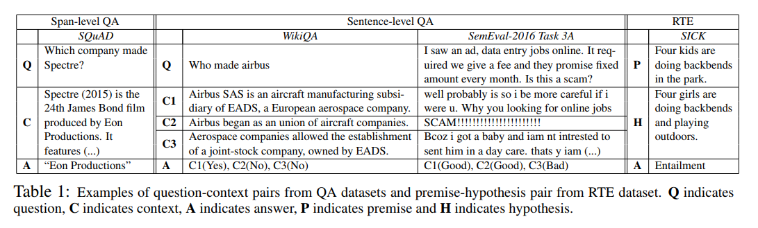
Here, I will give examples of different datasets.
| Dataset Name | Link | Suggested Metrics | Some Papers that use the dataset | Brief Description |
|---|---|---|---|---|
| WikiQA |
|
|
Question-Candidate_Answer1_to_N-Relevance1_to_N | |
| SQUAD 2.0 | Website |
|
QA-Transfer(for pretraining) | Question-Context-Answer_Range_in_context |
| Quora Duplicate Question Pairs |
|
Accuracy, F1 |
|
Q1-Q2-DuplicateProbablity |
| Sem Eval 2016 Task 3A | genism-data(semeval-2016-2017-task3-subtaskA-unannotated) |
|
QA-Transfer(SQUAD* MAP=80.2, MRR=86.4, P@1=89.1) |
Question-Comment-SimilarityProbablity |
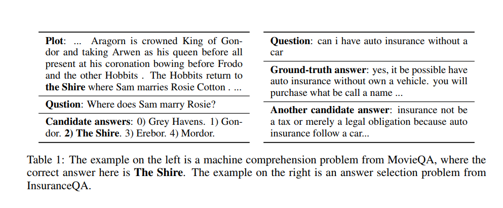
| MovieQA | Accuracy | SeqMatchSeq(SUBMULT+NN test=72.9%, dev=72.1%) |
Plot-Question-Candidate_Answers | |
| InsuranceQA | Website | Accuracy | SeqMatchSeq(SUBMULT+NN test1=75.6%, test2=72.3%, dev=77%) |
Question-Ground_Truth_Answer-Candidate_answer |
| SNLI | Accuracy |
|
Text-Hypothesis-Judgement | |
| TRECQA |
|
BiMPM(MAP:0.802, MRR:0.875) | Question-Candidate_Answer1_to_N-relevance1_to_N | |
| SICK | Website | Accuracy | QA-Transfer(Acc=88.2) | sent1-sent2-entailment_label-relatedness_score |
More dataset info can be found at the SentEval repo.
This dataset was originally released here
It has several different formats but at its base there is (for one data point):
- a question
- one or more correct answers
- a pool of all answers (correct and incorrect)
It doesn't have a simple format like question - document - relevance. So, we'll have to convert it to the QA format. That basically involves taking a question, its correct answer and marking it as relevant. Then for the remaining number of answers(however big you want the batch size to be), we pick (batch_size - current_size) from the pool of answers
The original repo has several files and is very confusing. Luckily, there is a converted version of it here
Since there is a pool of candidate answers from which a batch is sampled, the dataset becomes inherently stochastic.
Links to Papers:
While several models were cursorily checked, majorly, this study will have:
After going through the initial evaluation, we decided to implement the DRMM TKS model, since it gave the best score (0.65 MAP on WikiQA) with acceptable memory usage and time for training. The first model was considerable important since it set the standard for all other models to follow. I had to learn and implement a lot of Software Engineering principles like doctest, docstrings, etc. This model also helped me set up the skeleton structure needed for any Similarity Learning model. The code can be found here
- Iterate through the train set's sentences and develop your model's word2index dictionary(one index for each word). This is useful, especially when it comes to predicting on new data and we need to translate new sentences.
- Translate all the words into indexes using the above dict.
- Load a pretrained Embedding Matrix (like Glove) and reorder it so that its indices match with your word2index dictionary.
- There will be some words in the embedding matrix which aren't there in the train set. Although these extra embeddings aren't useful when it comes to training, they will be useful while testing and validating. So, append the word2index dict with these new words and reorder the embedding matrix accordingly.
- Make 2 additional entries in the embedding matrix for the pad word and the unkown word.
- Since all sentences won't be of the same shape, we will inevitably have to pad the sentences to the same length. You should decide at this point whether the pad vector is a zero vector or a random vector.
- While testing and validating, you will inevitably encounter an unkown word (a word not in your word2index dictionary). All these unkown words should be set to the same vector. Again, you can choose between a zero vector and a random vector.
- Once all the data is in the right format, we need to create a generator which will stream out batches of training examples (with padding added ofcourse). In the Question Answering context, there is a special consideration here. Usually, a training set will be of the form
[(q1, (d1, d2, d3), (q2, (d4, d5)))]with the releavnce labels like[(1, 0, 0), (0, 1)]. While setting up training examples, it's a good idea to make training pairs like [(q, d_rel), (q, d_not_relevant), (q, d_relevant), ...]. This "should" help the model learn the correct classification by contrasting relevant and non relevant answers. - Now that you batch generator is spitting out batches to train on, create a model, fix the loss, optimizer and other such parameters and train.
- The metrics usually reported by a library like Keras won't be very useful to evaluate your model as it trains. So, at the end of each epoch, you should set up your own callback as I have done here
- Once the model training is done, evaluate it on the test set. You can obviously use your own implementation, but as a standard, it would be better to write your results into the TREC format as I have done here and then use the
trec_evalbinary described before for evaluating. This standardizes evaluation and makes it easier for others to trust the result. - Saving models can get a bit tricky, especially if you're using keras. Keras prefers it's own way of saving against the satandard gensim
util.SaveLoadYou will have to save the keras model separate from the non-keras model and combine them while loading. Moreover, if you have any Lambda Layer, you will have to replace them with custom layers like I did here for the TopK Layer.
Most of the above has been done in my script and you can mostly just use that skeleton while changing just the _get_keras_model function.
Once my DRMM_TKS model was set up, it was performing very poorly (0.54 on MAP). After trying every idea I could imagine for fine tuning it, I ended up with a model which performed 0.63 on MAP. Beyond this point, however, I didn't feel like any changes I made would make it perform any better. You are welcome to try.
Seeing that DRMM_TKS wasn't doing so well, I moved my attention to the next best performing model in my list of model, MatchPyramid. This model, after some tuning, managed to score 0.64-0.65 MAP.
It was around this point that we came to the realization that the score wasn't much more than the baseline and a score of unsupervised baseline plus 0.15 would be needed to make it a worthwhile model to collect supervised data for.
I started looking for other datasets and happened to stumble upon the BiMPM paper which claimed a score of 0.71 on WikiQA. In it's score comparison table
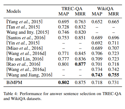
it had cited another paper SeqMatchSeq which claimed a further score of 0.74. I went about implementing BiMPM here and here which didn't perform as expected. I then ran the author's original code, where it unfortunately turned out that the author had reported the score on the dev set, not the test set (as per my run at least (with the author's random seeds)). (On asking the author in this issue, the author claims the split was test.) The actual test score was 0.69, not much more than the baseline for such a complicated model. I also found a pytorch implementation of SeqMatchSeq here in which there was an issue about MAP coming to 0.62 instead of 0.72 on dev set. The author commented:
I am afraid you are right. I used to reach
~72% via the given random seed on an old version of pytorch, but now with the new version of pytorch, I wasn't able to reproduce the result. My personal opinion is that the model is neither deep or sophisticated, and usually for such kind of model, tuning hyper parameters will change the results a lot (although I don't think it's worthy to invest time tweaking an unstable model structure). If you want guaranteed decent accuracy on answer selection task, I suggest you take a look at those transfer learning methods from reading comprehension. One of them is here https://github.com/pcgreat/qa-transfer
And thus, my hunt has lead me to the paper : Question Answering through Transfer Learning from Large Fine-grained Supervision Data which makes a crazier claim on MAP : 0.83 (On Ensemble of 12)
The paper's author provides the implementation here in tensorflow.
The author makes some notable claims in it's abstract:
We show that the task of question answering (QA) can significantly benefit from the transfer learning of models trained on a different large, fine-grained QA dataset. We achieve the state of the art in two well-studied QA datasets, WikiQA and SemEval-2016 (Task 3A), through a basic transfer learning technique from SQuAD. For WikiQA, our model outperforms the previous best model by more than 8%. We demonstrate that finer supervision provides better guidance for learning lexical and syntactic information than coarser supervision, through quantitative results and visual analysis. We also show that a similar transfer learning procedure achieves the state of the art on an entailment task.
So, how this model works is It takes an existing model for QA called BiDirectional Attention Flow (BiDAF), which would take in a query and a context. It would then predict the range/span of words in the context which is relevant to the query. It was adapted to the SQUAD dataset.
Example of SQUAD:
The QA-Transfer takes the BiDAF net and chops off the last layer to make it more QA like, ie., something more like WikiQA:
q1 - d1 - 0
q1 - d2 - 0
q1 - d3 - 1
q1 - d4 - 0
They call this modified network BiDAF-T
Then, they take the SQUAD dataset and break the context into sentences and labels each sentence as relevant or irrelevant. This new dataset is called SQUAD-T
How it works: SQUAD dataset is for span level QA
passage: "Bob went to the doctor. He wasn't feeling too good"
question: "Who went to the doctor"
span: "*Bob* went to the doctor. He wasn't feeling too good"
This can be remodelled such that:
question : "Who went to the doctor"
doc1 : "Bob went to the doctor."
relevance : 1 (True)

question : "Who went to the doctor"
doc2 : "He wasn't feeling too good"
relevance : 0 (False)
Effectively, we get a really big good dataset in the QA domain. The converted file is almost 110 MB.
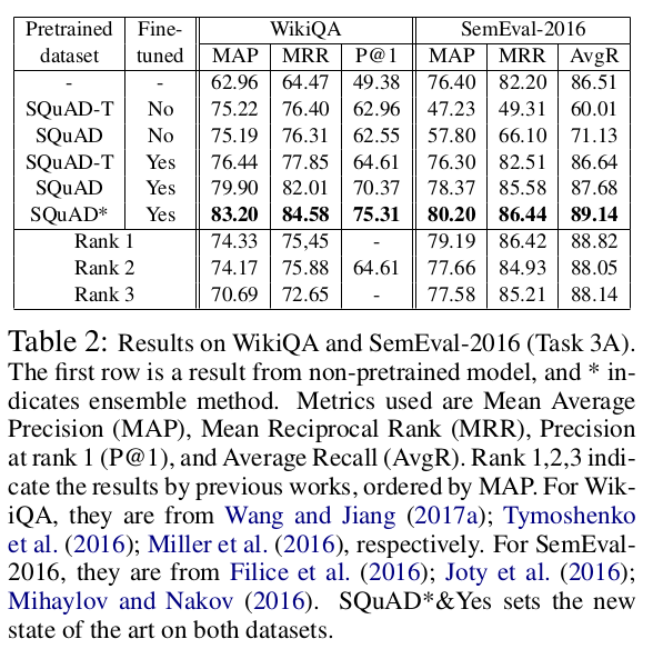
The new model, BiDAF-T is then trained on SQUAD-T. It gets MAP : 0.75 on WikiQA test set.
When BiDAF-T is finetuned on WikiQA, it gets MAP : 0.76
When BiDAF is trained on SQUAD, then the weights are transferred to SQUAD-T and it is further finetuned on WikiQA, it gets the MAP : 0.79
When it's done is an ensemble, it gets MAP : 0.83
They call it Transfer Learning.
So, as such, it's not exactly a new model. It's just an old model(BiDAF), trained on a modified dataset and then used on WikiQA and SentEval. However, the author claims that the model does suprisingly well on both of them. The author has provided their own repo.
Since, 0.79 feels like a good score, significantly (0.17) over the w2v baseline, I went about implementing it. You can find my implementation here and it is called using this eval script. Unfortunately, the scores don't perform as well.
Steps invovled:
I had to first convert the SQUAD dataset, a span level dataset, into a QA dataset. I have uploaded the new dataset and the script for conversion on my repo. I then trained the BiDAF-T model on the SQUAD-T dataset to check if it did infact reach the elusive score of
I got 0.64 on average (getting a 0.67 at one point) but this isn't more than MatchPyramid and it has several drawbacks:
Things to consider regarding QA Transfer/BiDAF:
- The original BiDAF code on SQUAD takes 20 hours to converge [reference]
- It is a very heavy model
- Since there is a QA Transfer from SQUAD, it won't work on non-english words. In that case, it's better to try an older method like BiMPM or SeqMatchSeq
List of existing implementations
- BiDAF code:
- BiDAF-T code:
In the tables below,
w2v/Glove Vec Averaging Baseline : refers to the score between 2 sentences calculated by averaging the word vectors(taken from Glove of Pennington et al) of their words and then taking the Cosine Similarity.
FT : refers to the same as above but using FastText
Glove + Regression NN : refers to getting sentence representations in the same way as above but using a single layer neural network with softmax activation
Glove + Multilayer NN : same as above but using a multilayer neural network instead of a single layer
| WikiQA test set | w2v 200 dim | FT 300 dim | MatchPyramid | DRMM_TKS | BiDAF only pretrain | BiDAF pretrain + finetune | MatchPyramid Untrained Model | DRMM_TKS Untrained Model | BiDAF Untrained Model |
|---|---|---|---|---|---|---|---|---|---|
| map | 0.6285 | 0.6199 | 0.6463 | 0.6354 | 0.6042 | 0.6257 | 0.5107 | 0.5394 | 0.3291 |
| gm_map | 0.4972 | 0.4763 | 0.5071 | 0.4989 | 0.4784 | 0.4986 | 0.3753 | 0.4111 | 0.2455 |
| Rprec | 0.4709 | 0.4715 | 0.5007 | 0.4801 | 0.416 | 0.4616 | 0.3471 | 0.3512 | 0.1156 |
| bpref | 0.4613 | 0.4642 | 0.4977 | 0.4795 | 0.4145 | 0.4569 | 0.3344 | 0.3469 | 0.1101 |
| recip_rank | 0.6419 | 0.6336 | 0.6546 | 0.6437 | 0.6179 | 0.6405 | 0.519 | 0.5473 | 0.3312 |
| iprec_at_recall_0.00 | 0.6469 | 0.6375 | 0.6602 | 0.648 | 0.6224 | 0.6441 | 0.5242 | 0.5534 | 0.3396 |
| iprec_at_recall_0.10 | 0.6469 | 0.6375 | 0.6602 | 0.648 | 0.6224 | 0.6441 | 0.5242 | 0.5534 | 0.3396 |
| iprec_at_recall_0.20 | 0.6469 | 0.6375 | 0.6602 | 0.648 | 0.6224 | 0.6441 | 0.5242 | 0.5534 | 0.3396 |
| iprec_at_recall_0.30 | 0.6431 | 0.6314 | 0.6572 | 0.648 | 0.6177 | 0.6393 | 0.5213 | 0.5515 | 0.3382 |
| iprec_at_recall_0.40 | 0.6404 | 0.6293 | 0.6537 | 0.6458 | 0.614 | 0.6353 | 0.5189 | 0.5488 | 0.3382 |
| iprec_at_recall_0.50 | 0.6404 | 0.6293 | 0.6537 | 0.6458 | 0.614 | 0.6353 | 0.5189 | 0.5488 | 0.3382 |
| iprec_at_recall_0.60 | 0.6196 | 0.6115 | 0.6425 | 0.6296 | 0.5968 | 0.6167 | 0.5073 | 0.5348 | 0.3289 |
| iprec_at_recall_0.70 | 0.6196 | 0.6115 | 0.6425 | 0.6296 | 0.5968 | 0.6167 | 0.5073 | 0.5348 | 0.3289 |
| iprec_at_recall_1t_recall_0.80 | 0.6175 | 0.6094 | 0.6401 | 0.627 | 0.594 | 0.6143 | 0.5049 | 0.5333 | 0.3263 |
| iprec_at_recall_0.90 | 0.6175 | 0.6094 | 0.6401 | 0.627 | 0.594 | 0.6143 | 0.5049 | 0.5333 | 0.3263 |
| iprec_at_recall_1.00 | 0.6175 | 0.6094 | 0.6401 | 0.627 | 0.594 | 0.6143 | 0.5049 | 0.5333 | 0.3263 |
| P_5 | 0.1967 | 0.1926 | 0.1967 | 0.1934 | 0.1984 | 0.2008 | 0.1704 | 0.1835 | 0.1473 |
| P_10 | 0.1119 | 0.1119 | 0.1156 | 0.1152 | 0.1128 | 0.1136 | 0.1095 | 0.1144 | 0.1033 |
| P_15 | 0.0787 | 0.0774 | 0.079 | 0.0785 | 0.0771 | 0.0779 | 0.0787 | 0.0787 | 0.0749 |
| P_20 | 0.0597 | 0.0591 | 0.0599 | 0.0591 | 0.0599 | 0.0599 | 0.0603 | 0.0601 | 0.0591 |
| Accuracy | |
|---|---|
| MatchPyramid | 69.20% |
| DRMM TKS | 68.49% |
| Glove Vec Averaging Baseline | 37.02% |
| Glove + Regression NN | 69.02% |
| Glove + Multilayer NN | 78 % |
| Accuracy | |
|---|---|
| MatchPyramid | 56.82% |
| DTKS | 57.00% |
| Glove + Regression NN | 59.68% |
| Glove + Multilayer NN | 66.18% |
| MatchPyramid Untrained Model | 23% |
| DTKS Untrained Model | 29% |
| Accuracy | |
|---|---|
| MatchPyramid | 53.57% |
| DRMM_TKS | 43.15% |
| MatchPyramid Untrained Model | 33% |
| DRMM_TKS Untrained Model | 33% |
| Glove + Regression NN | 58.60% |
| Glove + Multilayer NN | 73.06% |
Note: InsuranceQA is a "different dataset". It has a question, with one or two correct answers along with a pool of almost 500 incorrect answers. The InsuranceQA reader will, for a question randomly sample some incorrect answers to include in a batch. The dataset has been provided with 2 test sets (Test1 and Test2)
| IQA Test1 | w2v(300 dim) | MatchPyramid | DRMM_TKS |
|---|---|---|---|
| map | 0.6975 | 0.8194 | 0.5539 |
| gm_map | 0.5793 | 0.7415 | 0.4295 |
| Rprec | 0.5677 | 0.7246 | 0.3902 |
| bpref | 0.569 | 0.7296 | 0.3908 |
| recip_rank | 0.7272 | 0.8445 | 0.5901 |
| iprec_at_recall_0.00 | 0.7329 | 0.8498 | 0.5978 |
| iprec_at_recall_0.10 | 0.7329 | 0.8498 | 0.5978 |
| iprec_at_recall_0.20 | 0.7329 | 0.8498 | 0.5977 |
| iprec_at_recall_0.30 | 0.7316 | 0.8485 | 0.5944 |
| iprec_at_recall_0.40 | 0.7241 | 0.8416 | 0.5841 |
| iprec_at_recall_0.50 | 0.7238 | 0.8407 | 0.5838 |
| iprec_at_recall_0.60 | 0.6813 | 0.8055 | 0.5349 |
| iprec_at_recall_0.70 | 0.6812 | 0.8049 | 0.534 |
| iprec_at_recall_0.80 | 0.6662 | 0.7938 | 0.5185 |
| iprec_at_recall_0.90 | 0.6652 | 0.793 | 0.5171 |
| iprec_at_recall_1.00 | 0.6652 | 0.793 | 0.5171 |
| P_5 | 0.243 | 0.2663 | 0.2154 |
| P_10 | 0.1453 | 0.1453 | 0.1453 |
| P_15 | 0.0969 | 0.0969 | 0.0969 |
| P_20 | 0.0727 | 0.0727 | 0.0727 |
| P_30 | 0.0484 | 0.0484 | 0.0484 |
| P_100 | 0.0145 | 0.0145 | 0.0145 |
| P_200 | 0.0073 | 0.0073 | 0.0073 |
| P_500 | 0.0029 | 0.0029 | 0.0029 |
| P_1000 | 0.0015 | 0.0015 | 0.0015 |
| IQA Test2 | Word2Vec (300 dim) | MatchPyramid | DRMM_TKS |
|---|---|---|---|
| map | 0.7055 | 0.8022 | 0.5354 |
| gm_map | 0.589 | 0.714 | 0.4137 |
| Rprec | 0.5773 | 0.698 | 0.3725 |
| bpref | 0.58 | 0.7048 | 0.3704 |
| recip_rank | 0.7362 | 0.826 | 0.5698 |
| iprec_at_recall_0.00 | 0.7413 | 0.8318 | 0.5783 |
| iprec_at_recall_0.10 | 0.7413 | 0.8318 | 0.5783 |
| iprec_at_recall_0.20 | 0.7413 | 0.8316 | 0.5783 |
| iprec_at_recall_0.30 | 0.7402 | 0.8304 | 0.5757 |
| iprec_at_recall_0.40 | 0.7319 | 0.8243 | 0.5657 |
| iprec_at_recall_0.50 | 0.7317 | 0.8243 | 0.5652 |
| iprec_at_recall_0.60 | 0.6869 | 0.7903 | 0.5152 |
| iprec_at_recall_0.70 | 0.6866 | 0.7898 | 0.5147 |
| iprec_at_recall_0.80 | 0.6734 | 0.7771 | 0.5016 |
| iprec_at_recall_0.90 | 0.6731 | 0.7763 | 0.5011 |
| iprec_at_recall_1.00 | 0.6731 | 0.7763 | 0.5011 |
| P_5 | 0.2426 | 0.2602 | 0.2087 |
| P_10 | 0.1441 | 0.1441 | 0.1441 |
| P_15 | 0.096 | 0.096 | 0.096 |
| P_20 | 0.072 | 0.072 | 0.072 |
| P_30 | 0.048 | 0.048 | 0.048 |
| P_100 | 0.0144 | 0.0144 | 0.0144 |
| P_200 | 0.0072 | 0.0072 | 0.0072 |
| P_500 | 0.0029 | 0.0029 | 0.0029 |
| P_1000 | 0.0014 | 0.0014 | 0.0014 |
Fine tuning deep learning models can be tough, considering the model runtimes and the number of parameters.
Here, I will list some parameters to consider while tuning:
- The word vector dimensionality(50, 100, 200, 300) and source(Glove, GoogleNews)
- Dropout on different layers
- Making the Fully Connected/Dense layer deeper or wider
- Running lesser vs more epochs
- Bigger or Smaller Batch Sizes
While the models seem to be doing the best currently, they are a bit difficult to reproduce. There are several reasons I can imagine for that:
- Difference in Deep Learning Libraries and their versions used in implementations may vary or be outdated. Different libraries can have varying differences in small implementation details(like random initializations) which can lead to huge differences later on and are difficult to track.
- The large number of parameters coupled with it's stochastic nature means that the model's performance can vary greatly. Include the time it takes to get one result makes tuning them very very difficult to tune.
- "When a model doesn't perform well, is it because the model is wrong or is my implementation wrong?" This is a difficult question to answer.
My time spent with understanding, developing and testing Neural Networks for Similarity Learning has brought out the conclusions that:
- the current methods are not significantly better than a simple unsupervised word2vec baseline.
- the current methods are unreproducible/difficult to reproduce.
This work and effort has provided:
- a method to evaluate models
- implementations of some of the current SOTA models
- a list of datasets to evaluate models on and their readers
If anybody was to carry on with this work, I would recommend looking at the QA-Transfer model, which claims the current "State Of The Art". Although my implementation couldn't reproduce the result, I feel like there is some merit in the model. The reason for this belief is not based in QA-Transfer, but the underlying BiDAF model, which provides two demos which does really well. Since there is so much discrepancies in different implementations, it would be better to use the ported tf1.8 BiDAF
If you are looking to do "newer research", I would recommend you do what the authors of QA-Transfer did. They looked at the best performing model on the SQUAD 1.1 dataset, pretrained on it, removed the last layer and evaluated. Things have changed since: There is a newer better SQUAD (2.0) and that leader board has got a new "best" model. In fact, BiDAF model is no longer the best on SQUAD 1.1 or 2.0. Just take the current best model and do the pretraining!
If there's anything to take away from QA-Transfer, it's that span supervision and pretraining can be good ideas. This, especially, seems to be a new trend regarding Language Models