Predict tools in Galaxy workflows

How to execute the script

1. Execute the script extract_data.sh to extract two tabular files - tool-popularity.tsv and wf-connections.tsv. This script should be executed on a Galaxy instance's database (ideally should be executed by a Galaxy admin). There are two methods in the script one each to generate two tabular files. The first file (tool-popularity.tsv) contains information about the usage of tools per month. The second file (wf-connections.tsv) contains workflows present as the connections of tools. Save these tabular files.

2. Install the dependencies by executing the following lines:

   • conda env create -f environment.yml
   • conda activate tool_prediction

3. Execute the file train.sh. It has some input parameters:

   python <main python script> -wf <path to workflow file> -tu <path to tool usage file> -om <path to the final model file> -cd <cutoff date> -pl <maximum length of tool path> -ep <number of training iterations> -oe <number of iterations to optimise hyperparamters> -me <maximum number of evaluation to optimise hyperparameters> -ts <fraction of test data> -vs <fraction of validation data> -bs <range of batch sizes> -ut <range of hidden units> -es <range of embedding sizes> -dt <range of dropout> -sd <range of spatial dropout> -rd <range of recurrent dropout> -lr <range of learning rates> -ar <name of recurrent activation> -ao <name of output activation> -cpus <number of CPUs>

   Description of all parameters mentioned in the training script:

   • <main python script>: This script is the entry point of the entire analysis. It is present at scripts/main.py.

   • <path to workflow file>: It is a path to a tabular file containing Galaxy workflows. E.g. data/wf-connections.tsv.

   • <path to tool popularity file>: It is a path to a tabular file containing usage frequencies of Galaxy tools. E.g. data/tool-popularity.tsv.

   • <path to trained model file>: It is a path of the final trained model (h5 file). E.g. data/trained_model.hdf5.

   • <cutoff date>: It is used to set the earliest date from which the usage frequencies of tools should be considered. The format of the date is YYYY-MM-DD. This date should be in the past. E.g. 2017-12-01.

   • <maximum length of tool path>: This takes an integer and specifies the maximum size of a tool sequence extracted from any workflow. Any tool sequence of length larger than this number is not included in the dataset for training. E.g. 25.

   • <maximum number of evaluation to optimise hyperparameters>: The hyperparameters of the neural network are tuned using a Bayesian optimisation approach and multiple configurations are sampled from different ranges of parameters. The number specified in this parameter is the number of configurations of hyperparameters evaluated to optimise them. Higher the number, the longer is the running time of the tool. E.g. 30.

   • <number of iterations to optimise hyperparamters>: This number specifies how many iterations would the neural network executes to evaluate each sampled configuration. E.g. 10.

   • <number of training iterations>: Once the best configuration of hyperparameters has been found, the neural network takes this configuration and runs for "n_epochs" number of times minimising the error to produce a model at the end. E.g. 10.

   • <fraction of test data>: It specifies the size of the test set. For example, if it is 0.5, then the test set is half of the entire data available. It should not be set to more than 0.5. This set is used for evaluating the precision on an unseen set. E.g. 0.2.

   • <fraction of validation data>: It specifies the size of the validation set. For example, if it is 0.5, then the validation set is half of the entire data available. It should not be set to more than 0.5. This set is used for computing error while training on the best configuration. It should always be greater than 0.0. E.g. 0.2.

   • <range of batch sizes>: The training of the neural network is done using batch learning in this work. The training data is divided into equal batches and for each epoch (a training iteration), all batches of data are trained one after another. A higher or lower value can unsettle the training. Therefore, this parameter should be optimised. E.g. 1,128.

   • <range of hidden units>: This number is the number of hidden recurrent units. A higher number means stronger learning (may lead to overfitting) and a lower number means weaker learning (may lead to underfitting). Therefore, this number should be optimised. E.g. 1,128.

   • <range of embedding sizes>: For each tool, a fixed-size vector is learned and this fixed-size is known as the embedding size. This size remains same for all the tools. A lower number may underfit and a higher number may overfit. This parameter should be optimised as well. E.g. 1,128.

   • <range of dropout>: A neural network tends to overfit (especially when it is stronger). Therefore, to avoid or minimize overfitting, dropout is used. The fraction specified by dropout is the fraction of units "deleted" randomly from the network to impose randomness which helps in avoiding overfitting. This parameter should be optimised as well. E.g. 0.0,0.5.

   • <range of spatial dropout>: Similar to dropout, this is used to reduce overfitting in the embedding layer. This parameter should be optimised as well. E.g. 0.0,0.5.

   • <range of recurrent dropout>: Similar to dropout and spatial dropout, this is used to reduce overfitting in the recurrent layers (hidden). This parameter should be optimised as well. E.g. 0.0,0.5.

   • <range of learning rates>: The learning rate specifies the speed of learning. A higher value ensures fast learning (the optimiser may diverge) and a lower value causes slow learning (may not reach the optimum). This parameter should be optimised as well. E.g. 0.0001, 0.1.

   • <name of recurrent activation>: Activations are mathematical functions to transform input into output. This takes the name of an activation function from the list of Keras activations (https://keras.io/activations/) for recurrent layers. E.g. elu.

   • <name of output activation>: This takes the activation for transforming the input of the last layer to the output of the neural network. It is also taken from Keras activations (https://keras.io/activations/). E.g. sigmoid.

   • <number of CPUs>: This takes the number of CPUs to be allocated to parallelise the training of the neural network. E.g. 4.

   An example command: python scripts/main.py -wf data/workflow-connections-19-09.tsv -tu data/tool-popularity-19-09.tsv -om data/trained_model_sample.hdf5 -cd '2017-12-01' -pl 25 -ep 20 -oe 20 -me 50 -ts 0.0 -vs 0.2 -bs '1,512' -ut '1,512' -es '1,512' -dt '0.0,0.5' -sd '0.0,0.5' -rd '0.0,0.5' -lr '0.00001,0.1' -ar 'elu' -ao 'sigmoid' -cpus 4

4. The training of the neural network takes a long time (> 24 hours) for the complete data. Once the script finishes, h5 model file is created at the given location (path to trained model file).

5. Place the new model in the Galaxy repository at galaxy/database/trained_model.hdf5.

6. In the galaxy.yml config file, make the following changes:

   • Enable and then set the property enable_tool_recommendations to true
   • Enable and then set the property tool_recommendation_model_path to database/trained_model.hdf5

7. Now go to the workflow editor and choose any tool from the toolbox. Then, you can see a right-arrow in top-right of the tool. Click on it to see the recommended tools to be used after the previously chosen tool.

Tool prediction in action

Galaxy workflows as directed graphs

Galaxy workflow is a chain of (Galaxy) tools to process biological data. These datasets undergo a transformation at each node (a tool) which includes text manipulation, sorting on a column, deletion or addition of a column and so on. Each workflow can be considered as a directed acyclic graph where the output of each node becomes an input to the next node(s). Visit this website to see all the steps of workflow and its directed graph. Choose a workflow from the dropdown and see the Cytoscape graph. A typical workflow in Galaxy looks like this:

Predict tools

If a Galaxy user can see a list of possible next tool(s) at all stages of creating a workflow, it would be convenient and time-saving to create one. This work aims to achieve it by training a neural network on the existing set of workflows created by multiple users. There is a special kind of (recurrent) neural network, long short-term memory (LSTM), which learns connections in the input (sequential) data and predicts the next possible connections(s). The Galaxy workflows also qualify as sequential data (as a chain of tools) and this network is expected to work on these data processing pipelines to predict next possible connections. Moreover, this work aims towards creating a recommendation system for Galaxy workflows. The complete approach is explained below:

Suppose we have a workflow:

This workflow can be broken down into following smaller sequences (or training samples):

• pileometh > Remove beginning 1 (label)
• pileometh > Remove beginning 1 > Add_a_column1 (label)
• Add_a_column1 > cut1 > addValue (label)
• so on ...

The last item in each such path is a label (or category) of the previous sequence (of tools) which means that this label should be in the predicted set of next tools for that sequence. For example, "pileometh > Remove beginning 1" is a training sample and its label is "Add_a_column1". Following this way, each path is divided into training samples (a tool or a sequence of tools) and their labels. The logic behind this breaking up of a workflow is to make the classifier learn that if we are at a stage "pileometh > Remove beginning 1" of creating a workflow, the next tool would be "Add_a_column1". A similar approach is used for predicting words in sentences. Here, we can draw an analogy between our smaller sequences from workflows and smaller parts of sentences (in English for example). They are similar - sentences in a language like in English (I → want → to → go → to → Berlin) and our smaller sequences (filter1 → grouping1 → addvalue → join1) as both make sense only when their components are arranged in a particular order.

To feed these input training samples (smaller parts of workflows) into the neural network, we need to convert them into vectors (neural networks understand vectors and not words or text). In order to convert them into vectors, we create a list of unique nodes (tools) and assign them unique integers (let's call them an id for each node). Now, we take a training sample and identify its nodes, take their respective ids and arrange these integers in the same order as the original tool sequence. For example, let's take this small dummy workflow:

filter1 → grouping1 → addvalue → join1 → add_a_column1

Let's create a dictionary mapping a unique integer to each tool:

• { "addvalue": 1, "add_a_column1": 2, "filter1": 3, "join1": 4, "grouping1": 5 }

Now, create a training sample - a vector for the workflow:

• filter1 → grouping1 → addvalue → join1 (training sample)
• add_a_column1 (a label for the above part of the workflow)
• [ 0, 0,......, 0, 3, 5, 1, 4 ] (0s are added to make up for the maximum length of the input data).

Now, it's time for creating the label vector. It is a multi-hot encoded vector which means that this vector is all zeros except for the position(s) of the next tools. For example:

• [ 0, 0, 1, 0, 0 ] (a label vector for tool "add_a_column1" because its position value is 2 in the dictionary. So, the 3rd index of the vector is 1 and others are zeros).

If there are multiple labels for a training sample (which happens to be the case in this work), we add 1s to all the positions of the corresponding labels).

• [ 0, 1, 1, 0, 1 ] shows a multi-hot encoded label vector.

We create training samples and their labels in this manner and feed them to the network. The first layer in the network is an embedding layer which learns a dense, low dimensional vector for each training sample which is sparse. These dense, low dimensional vectors are then fed into the LSTM layer. Dropout is added between layers in order to avoid overfitting which happens when the learning (prediction performance) becomes better on training data and stops/saturates on test (unseen) data.

Data distribution

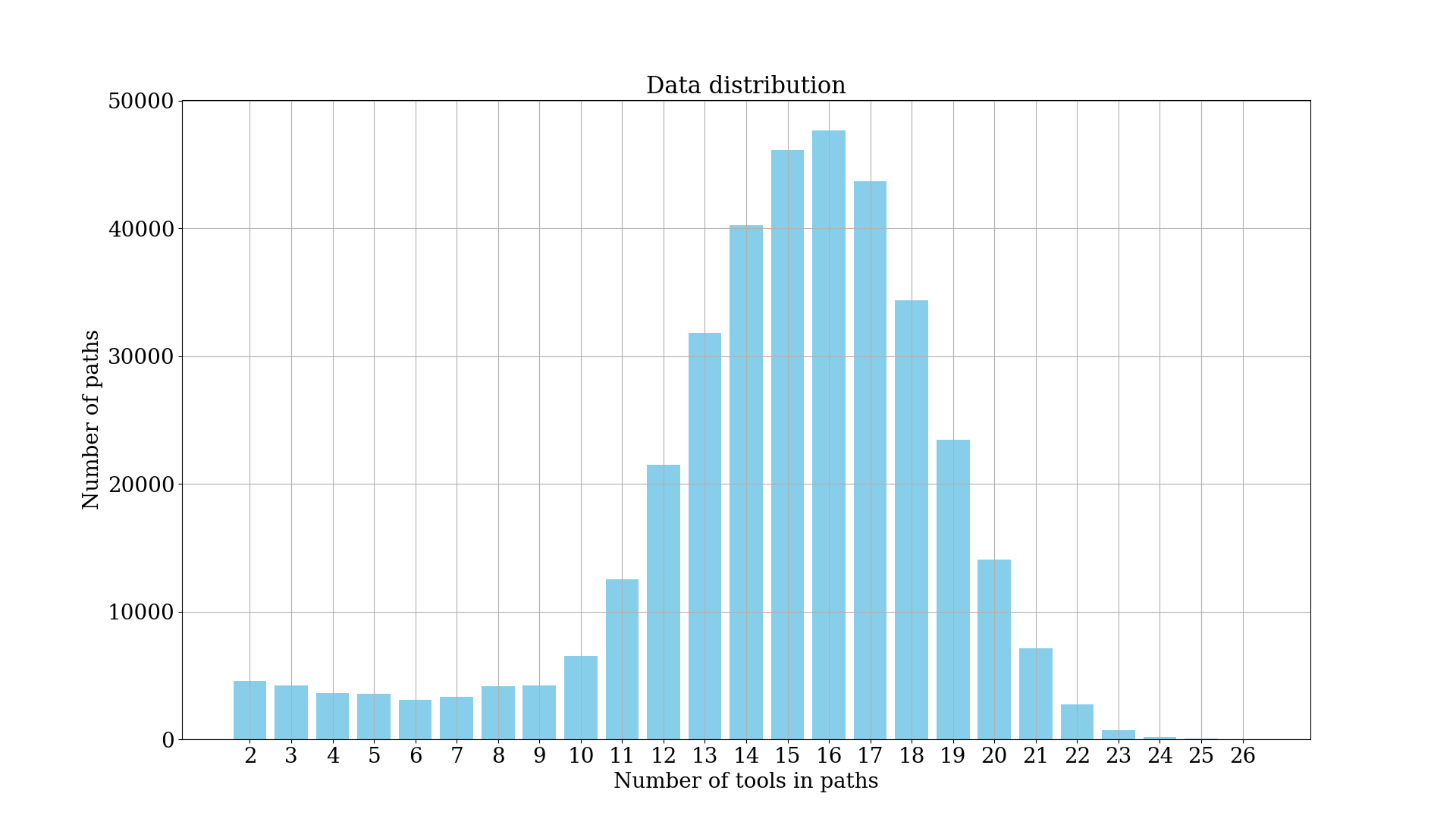
The above plot shows the distribution of the length of tool sequences. The length plays an important role to determine the dimensionality of the input dense vector. Thus, to reduce it, we take a maximum tool sequence length of 25.

Accuracy measure

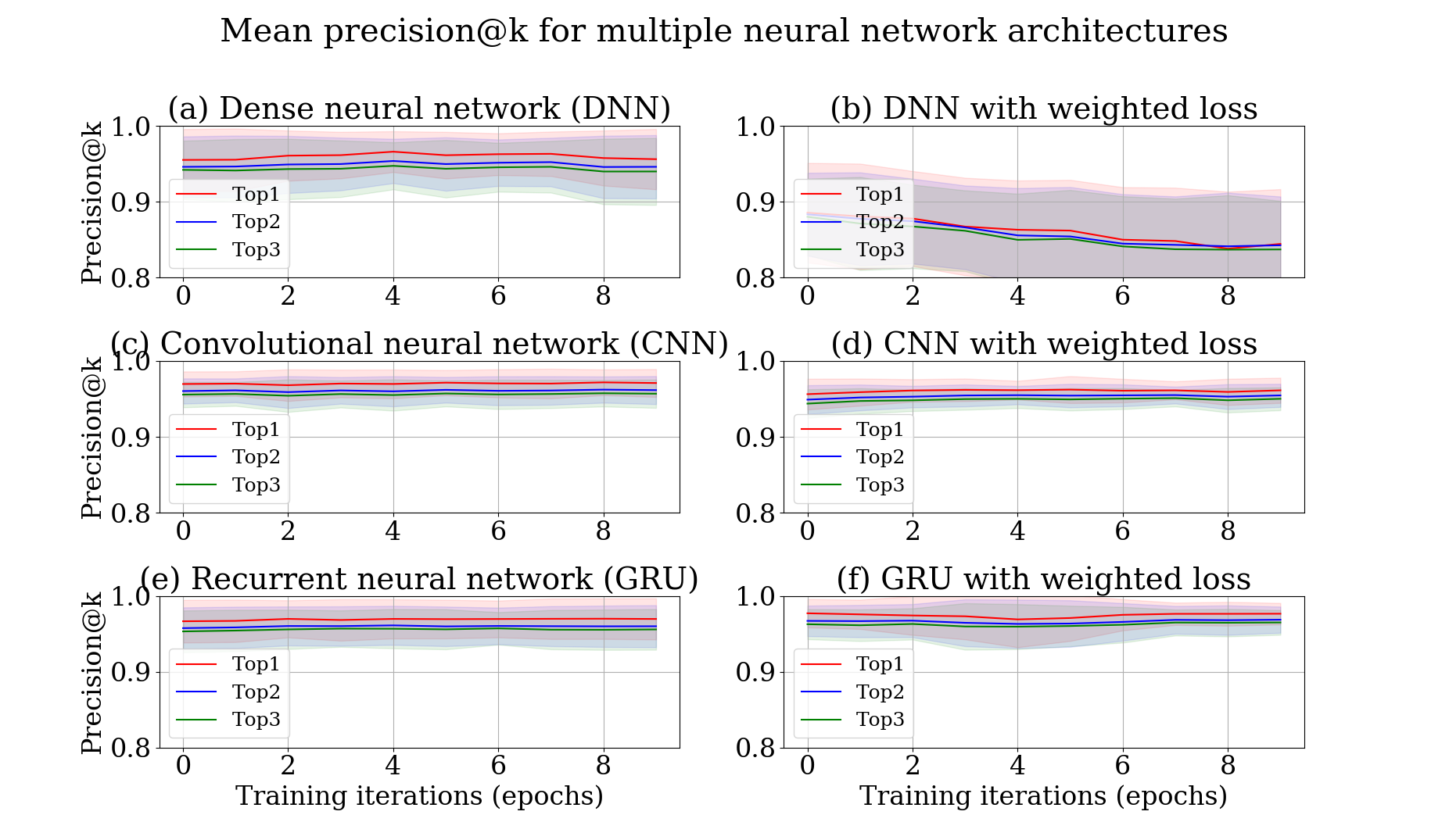
In the set of training sequences, each one can have many labels (or categories) which means that there can be multiple (next) tools for a sequence of tools. However, if we measure the accuracy of our approach which predicts just one next tool, it would be partially correct. Hence, we assess the performance on top k predicted tools (top-k accuracy). 20% of all samples are taken out for testing the trained model's performance and the rest is used to train the model.

Accuracy on test data

Precision comparison of different networks (Dense neural network (DNN), Convolutional (CNN) and Recurrent (RNN/GRU) neural networks)

Usage frequencies of predicted tools comparison of different networks (DNN, CNN and RNN/GRU)

Literature:

• LSTM
• A Beginner’s Guide to Recurrent Networks and LSTMs
• LSTM by Example using Tensorflow
• Learning to diagnose with LSTM Recurrent Neural Networks
• CNN-RNN: A Unified Framework for Multi-label Image Classification
• A Theoretically Grounded Application of Dropout in Recurrent Neural Network
• Empirical Evaluation of Gated Recurrent Neural Networks on Sequence Modeling
• Fast and Accurate deep network learning by exponential linear units(ELU)
• Recurrent Neural Network Regularization

Citations:

Cytoscape.js: a graph theory library for visualisation and analysis Franz M, Lopes CT, Huck G, Dong Y, Sumer O, Bader GD Bioinformatics (2016) 32 (2): 309-311 first published online September 28, 2015 doi:10.1093/bioinformatics/btv557 (PDF) PubMed Abstract