Advanced R Programming for Data Analysis

Some of the material is repurposed from the Data Carpentry lesson on Ecology, which is released under an open license.

Overview

The goal of this lesson is to orient intermediate R programmers and experienced programmers from other languages how to analyze data in R. R is commonly used in many scientific disciplines for statistical analysis. This workshop will focus on R as a general purpose programming language and data analysis tool, not on any specific statistical analysis.

It's always a challenge to balance the pace of this lesson.

Some of you are new to R and other may have been using R for some time.
As always, if you feel that I'm moving too fast, please interrupt me with your questions!
If you feel that I'm covering stuff you already know, please ask me questions that extend the topic.
I might also present an example without explanation and, instead, ask one of you to explain what is happening. If the answer seems obvious, please don't be offended! Look at it as an opportunity to check your own understanding by figuring out how to explain a complex idea to others.

Dependencies

You may want to make sure you have these packages install ahead of time.

install.packages(c('plyr', 'dplyr', 'tidyr', 'ggplot2'))

In this workshop, we will be using a subset of the Gapminder dataset. This is world-wide statistical data collected and curated to allow for a "fact based worldview." These data includes things like employment rates, birth rates, death rates, percent of GDP that's from agriculture and more. There are currently 519 variables overall, each as a time series.

You can see some examples of Gapminder's visualizations in this TED video. In this workshop, we'll focus just on life expectancy at birth and per-capita GDP by country, continent, and total population.

Introduction to RStudio

RStudio is what we would call an interactive development environment, or IDE, for the R programming language. It is interactive because we can issue it commands in the R language and the program responds with output. It is a development environment because we can use its features to develop scripts or programs in R that may consist of multiple R commands.

RStudio Layout

Open the RStudio program if you haven't already.

The interactive R console (left side of screen)
Workspace and history (tabbed in upper right)
Files/ Plots/ Packages/ Help (tabbed in lower right)

If we open a text file that contains an R program, what would we call an R script, a new pane would appear that displays the contents of that R script. R scripts are just plain text files but they have a *.R file extension to indicate that the contents should be interpreted as R commands.

Workflow in RStudio

The basis of programming is that we write down instructions for the computer to follow and then we tell the computer to follow those instructions. We call the instructions commands and we tell the computer to follow the instructions by executing or running those commands.

Generally speaking, there are two ways we can execute commands in RStudio. One way is to use RStudio interactively, as I alluded to earlier. That is, we can test R commands in the R console at the bottom right and maybe save those commands into an R script to run later. This works just fine but it can be tedious and error-prone. A better way would be for us to compose our R script in the file pane and then run the commands as a script or line-by-line.

To execute commands from the file pane in R, use the Run button at the top right.

Quick Overview of R

Let's quickly review programming in R so everyone's on the same page before we dive into more advanced topics.

Mathematical Operations in R

# Order of operations
3 + 5 * 2

# Parentheses help
(3 + 5) * 2

# Scientific notation
2/1000000
5e3

# Built-ins: Natural logarithm
log(1)

# Built-ins: Base-10 logarithm
log10(1)

# Getting help
?exp
??exponential

# Comparison operators
1 == 1
1 != 2
!TRUE
1 < 2
2 >= 1

Data Types

There are five (5) atomic data types in R. We can use the typeof() to determine the type of a data value.

# Double-precision (decimal numbers)
typeof(3.14159)

# Integers
typeof(5)
typeof(5L)

# Character strings
typeof("Hello, world!")

# Logical (Boolean)
typeof(TRUE)

# Complex numbers
typeof(2+3i)

Machine Precision

When performing numerical calculations in a programming environment like R, particularly when working with important quantities like money, it's important to be aware of how the computer represents decimal numbers. For various reasons we won't go into, computers typically only approximate decimal numbers when they're stored. If we don't guard against this, we may see some surprising results. Numbers that seem to be equal may actually have different underlying representations and therefore be different by a small margin of error (called machine numeric tolerance).

0.1 == 0.3 / 3

In general, don't use == to compare numbers unless they are integers. Instead, use the all all.equal function.

all.equal(0.1, 0.3 / 3)

Variables and Assignment

x <- 1/2

Variable names in R can contain any letters, numbers, the underscore, or the period character. R is probably the only programming language that allows you to use the period or dot character in a variable name. For this reason, some R experts advise against using such variable names.

x2 <- 3/4
my.parameter <- 'something'
my_parameter <- 'something else'

Using the right assignment operator is important. We may be tempted to use the = form because it is shorter, however, we should be aware of the important differences between these two operators.

# Argument assignment; no side effects
mean(x = 1:10)
x

# Variable assignment; side effects!
mean(x <- 1:10)
x

The above example may have you thinking that the = form is better to use in all cases. However, the following example shows a situation in which the = form is incorrectly interpreted as a keyword argument assignment.

df <- data.frame(foo = rnorm(10, 1000, 100))
within(df, bar = log10(foo)) # Breaks
within(df, bar <- log10(foo)) # Works

Functions

pow10 <- function (value) {
  10^value
}

pow10(1)

# Using the return() function
pow10 <- function (value) {
  return(10^value)
}

pow10(1)

# Chaining function application
pow10(log10(100))

Flow of Control

Note the difference between in keyword and %in% operator.

for (i in 1:10) {
  if (i %in% c(1, 3, 5, 7, 9)) {
    print(i)
  } else {
    print(0)
  }
}

Project Management with RStudio

The scientific process is naturally incremental and many projects start life as random notes, some code, then a manuscript, and, eventually, everything is a bit mixed together.

Link to "bad layout" figure.

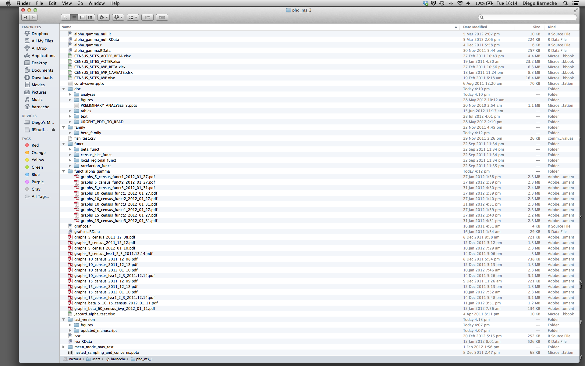
What's wrong with organizing a project like this?

It is really hard to tell which version of your data is the original and which is modified.
We may have multiple versions of our results and, here, the results are mixed together making it difficult to tell them apart at a glance.
It is difficult to relate the correct outputs, for example, a certain graph, to the exact code that has been used to generate it.

A good project layout, on the other hand, can make your life easier in so many ways:

It will help ensure the integrity of your data.
It makes it simpler to share your code with someone else.
It allows you to easily upload your code when submitting a manuscript for publication.
It makes it easier to pick the project back up after a break.

Here's one example.

Use the data/ folder to store your raw data and any intermediate datasets you may create. For the sake of transparency and scientific provenance, you should always keep your raw data around. Cleaning your data should be done with scripts that do not overwrite the original data. Therefore, the "cleaned" data should be kept in something like data_output.

Here's another example layout suggested by Daniel Chen.

project_root/
  doc/     # directory for documentation, one subdirectory for manuscript
  data/    # data for storing fixed data sets
  src/     # any source code
  bin/     # any compiled binaries or scripts
  results/ # output for tracking computational experiments performed on data
    20160701/
    20160705/
    ...

With version control on either the project root or the src directories. The data, results, and possibly the bin directories should be excluded from version control.

How RStudio Helps

RStudio has project management built- in. We'll use this today to create a self-contained, reproducible project.

Challenge: Create a self-contained project in RStudio.

Click the "File" menu button, then "New Project".
Click "New Directory".
Click "Empty Project".
Type in the name of the directory to store your 5. project, e.g. "my_project".
Make sure that the checkbox for "Create a git repository" is selected.
Click the "Create Project" button.

Now, when we start R in this project directory or when we open this project in RStudio, all of our work on this project will be entirely self-contained in this directory.

Best Practices

There is no single right way to organize a project but there are important best practices to follow.

Treat data as read only: This is probably the most important goal of setting up a project. Data is typically time consuming and/or expensive to collect. Working with the data interactively (e.g., in Microsoft Excel) where they can be modified means you are never sure of where the data came from or how it has been modified since collection. In science, we call this the problem of scientific provenance; keeping track of where our data came from and what we did to it in order to get some important result.
Data cleaning: In many cases, your initial data will be "dirty." That is, it needs significant pre-processing in order to coerce it into a format that R will find useful. This task is sometimes called "data munging." I find it useful to store these scripts in a separate folder and to create a second read-only data folder to hold the "cleaned" data sets.
Treat generated output as disposable: You should be able to regenerate all of your results from your R scripts. There are many ways to do this. I find it useful to have output folders with dates for names in YYYYMMDD format so that I can connect outputs to new developments in my research.

Challenge: Saving the Data to a New Directory

Using RStudio's project management pane at the lower-right, create a new folder called data inside your project folder. Then, copy the gapminder-FiveYearData.csv file to the new data directory.

Starting with Data Structures

Let's load in some data.

gapminder <- read.csv('data/gapminder-FiveYearData.csv')

Typically, the first thing we want to do after reading in some data is to take a quick look at it to verify its integrity.

head(gapminder)
tail(gapminder)

The default data structure in R for tabular data is referred to as a data frame. It has rows and columns just like a spreadsheet or a table in a database. A data frame is a collection of vectors of identical lengths. Each vector represents a column, and each vector can be of a different data type (e.g., characters, integers, factors).

In R, the columns of a data frame are represented as vectors. Vectors in R are a sequence of values with the same data type. We can use the c() function to create new vectors.

x1 <- c(1, 2, 3)
x2 <- c('a', 'b', 'c')

We can construct data frames as a collection of vectors using the data.frame() function. Note that if we try to put unlike data types in a single vector, they get coerced to the most flexible data type.

df <- data.frame(
  x1 = c(TRUE, FALSE, TRUE),
  x2 = c(1, 'red', 2))

A data structure in R that is very similar to vectors is the list class. Unlike vectors, lists can contain elements of varying data types and even varying classes.

list(99, TRUE 'balloons')
list(1:10, c(TRUE, FALSE))

A data frame is like a list in that it is a collection of multiple vectors, each with a different data type. We can confirm this with the str() function.

str(gapminder)

Challenge: Understanding Data Frames

Based on the output of the str() function, answer the following questions.

How many rows and columns are there in the data frame?
How many countries have been recorded in this data frame?
How many continents have been recorded in this data frame?

As you can see, many of the columns consist of integers, however, the columns country and continent are of a special class called factor. Before we learn more about the data.frame class, let's talk about factors.

Factors

Factors...

Are used to represent categorical data;
Can be ordered or unordered.

Understanding them is necessary for statistical analysis and for plotting. Factors are stored as integers, and have labels associated with these unique integers. While factors look (and often behave) like character vectors, they are actually integers under the hood, and you need to be careful when treating them like strings.

Once created, factors can only contain a pre-defined set of values, known as levels. By default, R always sorts levels in alphabetical order. For instance, if you have a factor with 2 levels:

times <- factor(c('night', 'day', 'night', 'day'))

R assigns the day level the integer value 1 even through night appears first in the vector. We can confirm this and the number of levels using two functions.

levels(times)
nlevels(times)

By default, factors are unordered, which makes some kinds of comparison and aggregation meaningless.

spice <- factor(c('low', 'medium', 'low', 'high'))
levels(spice)
max(spice)

In calling factor(), we can specify the labels explicitly with the levels keyword argument, however...

spice <- factor(c('low', 'medium', 'low', 'high'),
  levels = c('low', 'medium', 'high'))
levels(spice)

...If we specify ordered=TRUE when we set the factor levels, we can now talk about the relative magnitudes of categories.

spice <- factor(c('low', 'medium', 'low', 'high'),
  levels = c('low', 'medium', 'high'), ordered = TRUE)
max(spice)

Setting the order of the factors can be crucial in linear regression, where the reference level of a categorical predictor is the first level of a factor. Factors allow us to order and compare categorical data with human-readable labels instead of storing the field as ambiguous integers.

Converting Factors

If you need to convert a factor to a character vector, you use the as.character() function. However, if the levels of the factor appear as numbers, such as concentration levels, then conversion to a numeric vector can be tricky. One method is to convert factors to characters and then numbers. Another method is to use the levels() function. Compare:

f <- factor(c(1, 5, 10, 2))
as.numeric(f)
as.numeric(as.character(f))
as.numeric(levels(f))[f]

Notice that in the levels() approach, three important steps occur:

We obtain all the factor levels using levels(f);
We convert these levels to numeric values using as.numeric(levels(f));
We then access these numeric values using the underlying integers of the vector f inside the square brackets.

Challenge: Tabulation

The function table() tabulates and cross-tabulates observations. Tabulation can be used to create a quick bar plot of your data. In this case, we can quickly plot the number of observations in each continent in the data. Answer the following questions after tabulating and plotting the continents in the Gapminder data.

tabulation <- table(gapminder$continent)
tabulation
barplot(tabulation)

In which order are the continents listed?
How can you re-order the continents so that they are plotted in order of highest frequency to lowest frequency (from left to right)?

Cross Tabulation

Cross tabulation can aid in checking the assumptions about our dataset. Cross tabulation tallies the number of corresponding rows for each pair of unique values in two vectors. Here, we can use it to check that the expected number of records exist for each continent in each year. Because each country appears only once a year, these numbers correspond to the number of countries recorded for that continent in that year.

table(gapminder$year, gapminder$continent)

To avoid re-writing gapminder multiple times in this function call, we can use the helper function with.

with(gapminder, table(year, continent))

The with function signals to R that the names of variables like year and continent can be found among the columns of the gapminder data frame. Writing our cross-tabulation this way makes it easier to read at a glance.

Data Frames

By default, when building or importing a data frame, the columns that contain characters (i.e., text) are coerced (converted) into the factor data type. Depending on what you want to do with the data, you may want to keep these columns as character. To do so, read.csv() and read.table() have an argument called stringsAsFactors which can be set to FALSE.

gapminder2 <- read.csv('data/gapminder-FiveYearData.csv', stringsAsFactors = FALSE)
str(gapminder2)

If you want to set this behavior as the new default throughout your script, you can set it in the options() function.

options(stringsAsFactors = FALSE)

If you choose to set any options(), make sure you do so at the very top of your R script so that it is easy for others to see that you're deviating from the default behavior of R.

There are several questions we can answer about our data frames with built-in functions.

dim(gapminder)
nrow(gapminder)
ncol(gapminder)
names(gapminder)
rownames(gapminder)
summary(gapminder)

Most of these functions are "generic;" that is, they can be used on other types of objects besides data.frame.

Sequences and Indexing

Recall that in R, the colon character is a special function for creating sequences.

1:10

This is a special case of the more general seq() function.

seq(1, 10)
seq(1, 10, by = 2)

Integer sequences like these are useful for extracting data from our data frames. Our survey data frame has rows and columns (it has 2 dimensions), if we want to extract some specific data from it, we need to specify the "coordinates" we want from it. Row numbers come first, followed by column numbers.

# First column of gapminder
gapminder[1]

# First element of first column
gapminder[1, 1]

# First element of fifth column
gapminder[1, 5]

# First three elements of the fifth column
gapminder[1:3, 5]

# Third row
gapminder[3, ]

# Fifth column
gapminder[, 5]

# First six rows
gapminder[1:6, ]

We can also use negative numbers to exclude parts of a data frame.

# The first column removed
head(gapminder[, -1])

# The second through fourth columns removed
head(gapminder[, -2:-4])

Recall that to subset the data frame's entire columns we can use the column names.

gapminder['year']   # Result is a data frame
gapminder[, 'year'] # Result is a vector
gapminder$year      # Result is a vector

Challenge

The function nrow() on a data.frame returns the number of rows. Use it, in conjunction with seq() to create a new data.frame that includes every 10th row of the gapminder data frame starting at row 10 (10, 20, 30, ...).

Checkpoint: Data Structures in R

Now you should be familiar with the following:

The different types of data in R.
The different data structures that we can use to organize our data in R.
How to ask basic questions about the structure and size of our data in R.

Subsetting and Aggregating Data

The Gapminder data contain surveys of each country's per-capita GDP and life expectancy every five years. Let's learn how to use R's advanced data manipulation and aggregation features to answer a few questions about the Gapminder data.

Which countries had a life expectancy lower than 30 years of age in 1952?
What was the mean per-capita GDP between 2002 and 2007 for each country?
What is the range in life expectancy for each continent?

To answer these questions, we'll combine relatively simple tasks in R together, progressively building towards a more complex answer.

Subsetting Data Frames

To answer our first question, we need to learn about subsetting data frames. Recall our comparison operators; we want to find those entries of the lifeExp column that are less than 30.

gapminder$lifeExp < 30

That's a lot of output! In fact, there's one logical value for every row in the data frame. This makes sense; we basically performed a calculation on the lifeExp column, comparing every value in that column to 30. The result is a logical vector with TRUE wherever the lifeExp value is less than 30 and FALSE elsewhere.

Thus, when we subset the rows of gapminder with this logical vector, we obtain only those rows that matched. Finally, we specified we just wanted the country column in this result.

gapminder[gapminder$lifeExp < 30, 'country']

This is the best way to subset data frames when we're writing a reusable R script. However, when we're using R interactively as part of exploratory data analysis, it may be easier to use the subset() function.

subset(gapminder, lifeExp < 30, select = 'country')

Note that, unlike our bracket notation, the subset() function returns a data frame for an input data frame.

The aggregate() Function

To answer the other questions we asked, we need to be able to summarize values in one column for each of the unique values in another column. That is, we need to aggregate our data, and there's a built-in function in R to do just this.

?aggregate

Note that the by argument in aggregate() takes a list of unique values "as long as the variables in the data frame x." This means we can call aggregate() on two separate vectors, even if we don't have a data frame, as long as those vectors are the same length. Recall that we wanted to know the mean per-capita GDP between 2002 and 2007 for each country. Thus, we need to start by subsetting the gapminder data frame to just those years.

gm.subset <- gapminder[gapminder$year %in% c(2002, 2007),]

Now we can provide the column the be aggregated, gdpPercap, and the column with the unique group values, country, to the aggregate() function.

aggregate(gm.subset$gdpPercap, by = list(gm.subset$country), FUN = mean)

Function Application

Another way we can aggregate data in R is with function application. R has several built in functions like sapply(), tapply(), and apply() that apply a function over a list, vector, or data frame.

Of these functions, sapply() is the simplest. We can use it, for instance, with the class() function to check the data type of every column in our data frame. Because a data frame is really a list of vectors, sapply() applies the class() function to each vector.

sapply(gapminder, class)

With the more general apply() function, we can aggregate across the rows or columns of a data frame. We have to tell apply() which we're aggregating over, however: rows or columns.

?apply

This is the MARGIN argument of apply(). Recall that when indexing data frames, we specify the row index before the column index. Thus, the number 1 is the margin for row application and the number 2 is for column application. For instance, we can reproduce the sapply() example with apply() like so.

apply(gapminder, 2, class)

We can also calculate summary statistics over multiple numeric columns, such as the last two columns of gapminder.

apply(gapminder[,5:6], 2, mean)

However, this kind of aggregation isn't very meaningful for this dataset. We probably don't care about the mean life expectancy or per-capita GDP across a period of over 50 years. Instead, we'd like to summarize columns within predefined groups, like countries or continents. This is where tapply() comes in.

?tapply()

We can see that, like aggregate(), we can specify the groups to aggregate within. Let's reproduce our result from aggregate() starting with the subset data, gm.subset.

tapply(gm.subset$gdpPercap, gm.subset$country, FUN = mean)

Note that this output is formatted differently. This is because, unlike aggregate() which returns a vector, tapply() simplifies the data by default and returns an instance of the array class, a more general kind of vector.

In addition to the built-in functions like mean(), we can provide any custom function to tapply(). For instance, we can use it to answer Question 3; to find out how much life expectancy varies across each continent in 2007. Here, we use the with() function to subset our data before calling tapply().

with(gapminder[gapminder$year == 2007,], tapply(lifeExp,
  INDEX = continent, FUN = function (values) {
    max(values) - min(values)
    }))

Analyzing Data with dplyr

Because the R programming language is open source, the developer community moves quickly and a number of different tools are available for a wide variety of tasks. We'll now explore some additional tools available in third-party libraries developed by the R community. R packages are basically sets of additional functions that let you do more stuff. The functions we’ve been using so far, like str() or data.frame(), come built into R; packages give you access to more of them.

Before you use a package for the first time you need to install it on your machine, and then you should import it in every subsequent R session when you need it. R packages can be installed using the install.packages() function. Let's try to install the dplyr package, which provides advanced data querying and aggregation.

install.packages('dplyr')

Now that we've installed the package, we can load it into our current R session with the library() function.

library(dplyr)

What is dplyr?

The package dplyr provides easy tools for the most common data manipulation tasks. It is built to work directly with data frames. dplyr can perform fast manipulations on relatively large datasets because much of the underlying code is written in C++ and compiled to binaries that connect to R. An additional feature is the ability to work directly with data stored in an external database. The benefits of doing this are that the data can be managed natively in a relational database, queries can be conducted on that database, and only the results of the query returned.

This addresses a common problem with R in that all operations are conducted in memory and thus the amount of data you can work with is limited by available memory. The database connections essentially remove that limitation in that you can have a database of many 100s of gigabytes, conduct queries on it directly, and pull back just what you need for analysis in R.

Selecting and Filtering with dplyr

We're going to learn some of the most common dplyr functions: select(), filter(), mutate(), group_by(), and summarize().

To select columns from a data frame, use select(). The first argument to this function is the data frame (gapminder), and the subsequent arguments are the columns to keep.

output <- select(gapminder, country, pop)
head(output)

To choose rows, use filter().

filter(gapminder, country == 'Australia')

Pipes

But what if you wanted to select and filter at the same time? There are three ways to do this, two of which we've already seen:

Use intermediate steps; recall how we would save a subset of our data frame as a new, temporary data frame. This can clutter up our workspace with lots of objects.
Nested functions; we saw this most recently with the with() function. This is handy, but can be difficult to read if too many functions are nested together.
Pipes.

The last option, pipes, are a fairly recent addition to R. Pipes let you take the output of one function and send it directly to the next, which is useful when you need to do many things to the same data set. In R, the pipe operator, %>%, is available in the magrittr package, which is installed as part of dplyr. Let's get some practice using pipes.

gapminder %>%
  filter(continent == 'Oceania') %>%
  select(country, year, pop)

If we want to save the output of this pipeline, we can assign it to a new variable.

oceania <- gapminder %>%
  filter(continent == 'Oceania') %>%
  select(country, year, pop)

Challenge: Pipes

Using pipes, subset the gapminder data to the United States and retain the year, population, and life expectancy columns.

Mutating Data with dplyr

Frequently you'll want to create new columns based on the values in existing columns, for example to do unit conversions, or find the ratio of values in two columns. For this we'll use mutate(). For instance, we can convert per-capita GDP to total GDP as follows.

gapminder %>%
  mutate(gdp = gdpPercap * pop)

Woops. This is a lot to look at. Luckily, we can pipe the results into the head() function.

gapminder %>%
  mutate(gdp = gdpPercap * pop) %>%
  head()

Challenge: One-Step Mutation

Mutate the gapminder data so that there are two new columns, the base-10 logarithm of population and the base-10 logarithm of per-capita GDP. Note there are two ways to do this in dplyr.

Split-Apply-Combine with dplyr

dplyr introduces the split, apply, combine workflow to our skill set. This workflow allows us to split apart a data frame based on the levels (or unique values) of one or more columns, apply a function to those subgroups, and combine the results together.

To split the data, we need to introduce the group_by function. group_by() is often used together with summarize(), which collapses each group into a single-row summary of that group. group_by() takes as argument the column names that contain the categorical variables for which you want to calculate the summary statistics. For instance, to view the maximum life expectancy by country in 2007:

gapminder %>%
  group_by(country) %>%
  summarize(max(lifeExp))

We can see that the output appears truncated; instead of running off the screen, we get just the first few rows and a count of how many remain to be seen. That's because dplyr, instead of a data.frame, has returned an instance of the tbl_df class. This is a data structure that's very similar to a data frame; for our purposes the only difference is that it won't automatically show too many rows. It also displays the data type for each column under its name. If you want to display more data on the screen, you can add the print() function at the end with the argument n specifying the number of rows to display.

gapminder %>%
  group_by(country) %>%
  summarize(max(lifeExp)) %>%
  print(n = 15)

What happens when we use mutate() instead of summarize() after a group_by() step? While summarize() returns exactly one value for every group, mutate() will return a value for all the rows within a group, but it will still perform that calculation over only the rows within the group. Compare the following two examples to the one above:

# Calculates max life expectancy across ALL countries, all years
gapminder %>%
  mutate(max.lifeExp = max(lifeExp)) %>%
  print(n = 15)
  
# Calculates max life expectancy for each country, across all years;
#   returns the same value (max life expectancy for the respective country)
#   for all rows
gapminder %>%
  group_by(country) %>%
  mutate(max.lifeExp = max(lifeExp)) %>%
  print(n = 15)

Tabluation (Counting Rows)

We can perform tabulation using the tally() function. How many countries are found in each continent in 2007?

gapminder %>%
  filter(year == 2007) %>%
  group_by(continent) %>%
  tally()

We can even bring some base R functions into our pipeline. For instance, we can investigate a possible correlation between mean per-capita GDP and mean life expectancy over the past 50 years.

gapminder %>%
  group_by(country) %>%
  summarize(y = mean(lifeExp), x = mean(gdpPercap)) %>%
  select(x, y) %>%
  plot(main = 'Life Expectancy vs. Per-Capita GDP',
    xlab = 'Mean Per-Capita GDP', ylab = 'Mean Life Expectancy')

Let's try taking the base-10 logarithm of mean per-capita GDP.

gapminder %>%
  group_by(country) %>%
  mutate(log.gdpPercap = log10(gdpPercap)) %>%
  summarize(y = mean(lifeExp), x = mean(log.gdpPercap)) %>%
  select(x, y) %>%
  plot(main = 'Life Expectancy vs. Per-Capita GDP',
    xlab = 'Mean Log10 Per-Capita GDP', ylab = 'Mean Life Expectancy')

Cleaning Data with tidyr

There's one more question I want to answer about the gapminder data using pipes. How much did life expectancy change in each African country in the 40-year period between 1952 and 1992? This is going to be harder to answer than our previous questions because of how our data are structured. We can't use summarize() here because there is no way to distinguish between the years when we're aggregating values in a given column. We could assume that life expectancy increased in all cases and simply subtract the minimum value from the maximum value but our assumption may not hold; there might be some places where life expectancy, for whatever reason, decreased.

The tidyr package in R has some additional functions for data cleaning and restructuring that can be combined with the pipelines we introduced in dplyr.

install.packages('tidyr')

Following best practices, we'll build this analysis by starting with small parts that we understand. We know that we want to filter the data to the African continent and to the years 1952 and 1992.

gapminder %>%
  filter(continent == 'Africa') %>%
  filter(year %in% c(1952, 1992)) %>%
  head()

If we break out the value of life expectancy for each year into its own columns, we can then simply use mutate to subtract the life expectancy in 1952 from the life expectancy in 1992. This is what the spread() function does in the tidyr package.

library(tidyr)
gapminder %>%
  filter(continent == 'Africa') %>%
  filter(year %in% c(1952, 1992)) %>%
  spread(year, lifeExp, sep = '.') %>%
  head()

From this output, it looks like we now have separate columns but the rows need to be collapsed into one entry per country. We could do this with summarize() but there is an easier way. It turns out that spread() is pretty smart about this, we just need to ensure that the only variables in our data frame are the "key" and "value" variables and any non-unique grouping variable, like country. So, we select() these variables before we spread().

gapminder %>%
  filter(continent == 'Africa') %>%
  filter(year %in% c(1952, 1992)) %>%
  select(country, year, lifeExp) %>%
  spread(year, lifeExp, sep = '.') %>%
  head()

Now we're ready to calculate the difference between the two years.

gapminder %>%
  filter(continent == 'Africa') %>%
  filter(year %in% c(1952, 1992)) %>%
  select(country, year, lifeExp) %>%
  spread(year, lifeExp, sep = '.') %>%
  mutate(life.exp.change = year.1992 - year.1952) %>%
  head()

We can use the arrange() function to sort the output by a particular field. In this case, we want to look at those countries with the lowest gain in life expectancy at the top.

gapminder %>%
  filter(continent == 'Africa') %>%
  filter(year %in% c(1952, 1992)) %>%
  select(country, year, lifeExp) %>%
  spread(year, lifeExp, sep = '.') %>%
  mutate(life.exp.change = year.1992 - year.1952) %>%
  arrange(life.exp.change) %>%
  head()

Checkpoint: Data Analysis in R

Now you should be familiar with the following:

How to read in a CSV as an R data.frame
Factors and when to use them
Tabulation and cross-tabulation for checking assumptions about your data
Numeric sequences for indexing vectors and data frames
Subsetting data frames
Aggregating data frames with aggregate() or apply()
The split-apply-combine workflow
How to use dplyr and pipes in a data analysis workflow

Next, you'll see how to create plots of your data for checking assumptions, validating the data, and answering data analysis questions.

Data Visualization in R

Disclaimer: We will be using the functions in the ggplot2 package. R has powerful built-in plotting capabilities, but for this exercise, we will be using the ggplot2 package, which facilitates the creation of highly-informative plots of structured data.

ggplot2 is a plotting package that makes it simple to create complex plots from data in a dataframe. It uses default settings, which help creating publication quality plots with a minimal amount of settings and tweaking. The "gg" in ggplot2 refers to the "grammar of graphics," which is a design philosophy for how to describe visualizations with computer code.

ggplot graphics are built step-by-step by adding new elements; in the ggplot2 documentation, these elements include what are called "geometric objects," which are things like points, lines, and polygons that correspond to your data. We'll first use ggplot2 to create a plot of life expectancy versus per-capita GDP. To create this plot with ggplot2 we need to:

Bind the plot to a specific data frame using the data argument;
Define aesthetics (aes) that map variables in teh data to axes on the plot or to plotting size, shape, color, etc.;
Add geometric objects; the graphical representation of the data in the plot (points, lines, polygons). To add a geometric objector or geom, use the + operator.

ggplot(data = gapminder)

If this is all we instruct R to do, we see that the "Plots" tab in RStudio has appeared and a background has been rendered but nothing else. Basically, ggplot2 has set up a plotting environment but nothing more.

ggplot(data = gapminder, aes(x = gdpPercap, y = lifeExp))

After we add the aesthetics, we can see that the x and y axes have been set up with the appropriate ranges and drawn on the plot along with a grid that defines the coordinate space they span.

ggplot(data = gapminder, aes(x = gdpPercap, y = lifeExp)) +
  geom_point()

After adding a point layer, we can see the data plotted.

The + in the ggplot2 package is particularly useful because it allows us to modify existing ggplot objects. This means we can easily set up plot "templates" and conveniently explore different types of plots, so the above plot can also be generated with code like this:

base <- ggplot(data = gapminder, aes(x = gdpPercap, y = lifeExp))
base + geom_point()

Some things to note:

Anything you put in the ggplot() function can be seen by any geom layers that you add. i.e. these are universal plot settings. This includes the x and y axis you set up in aes().
You can also specify aesthetics for a given geom independently of the aesthetics defined globally in the ggplot() function.

ggplot(data = gapminder) +
  geom_point(aes(x = gdpPercap, y = lifeExp))

Building Plots Iteratively

Building plots with ggplot2 is typically an iterative process. We start by defining the dataset we'll use, lay the axes, and choose a geometric object.

ggplot(data = gapminder, aes(x = gdpPercap, y = lifeExp)) +
  geom_point()

Then, we start modifying this plot to extract more infromation from it. For instance, we can add transparency (alpha) to avoid overplotting.

ggplot(data = gapminder, aes(x = gdpPercap, y = lifeExp)) +
  geom_point(alpha = 0.3)

We can also add a color to the point. Note that when these options are set outside of the aesthetics (outside of the aes() function), they apply uniformly to all data points, whereas those inside the aesthetics vary with the values in the data.

ggplot(data = gapminder, aes(x = gdpPercap, y = lifeExp)) +
  geom_point(alpha = 0.3, color = 'blue')

If we want color to vary with the values in our data frame, we need to assign a column of the data frame as the source for those values and then map those values onto an aesthetic within the aes() function. For instance, let's let color vary by continent.

ggplot(data = gapminder, aes(x = gdpPercap, y = lifeExp)) +
  geom_point(alpha = 0.3, aes(color = continent))

Challenge: Changing the Scale

In many types of data, it is important to consider the scale of the observations. For example, it may be worth changing the scale of the axis to better distribute the observations in the space of the plot. Changing the scale of the axes is done similarly to adding/modifying other components (i.e., by incrementally adding commands). Represent per-capita GDP on a log-10 scale. For a hint, look up the help documentation on scale_x_log10().

Boxplots

With ggplot2 we can easily create more sophisticated plots than a scatter plot. For instance, let's explore the distribution of life expectancy across continents.

ggplot(data = gapminder, aes(x = continent, y = lifeExp)) +
  geom_boxplot()

By adding points to the same plot, we can get a better idea of the number of measurements and of their distribution.

ggplot(data = gapminder, aes(x = continent, y = lifeExp)) +
  geom_boxplot() +
  geom_point()

This isn't quite what we wanted. Because all the points are plotted at the same x axis coordinate, we're not realizing any value in plotting both the points and the box plots. We can "jitter" the points in one direction so they are easier to see. We can also disable the background fill of the boxplots for clarity.

ggplot(data = gapminder, aes(x = continent, y = lifeExp)) +
  geom_boxplot(alpha = 0) +
  geom_jitter(alpha = 0.5, color = 'tomato')

Challenge: Violin Plot

Boxplots are useful summaries, but hide the shape of the distribution. For example, if there is a bimodal distribution, this would not be observed with a boxplot. An alternative to the boxplot is the violin plot (sometimes known as a beanplot), where the shape (of the density of points) is drawn. Replace the box plot with a violin plot. For a hint, look up the help documentation on geom_violin().

?geom_violin

Plotting Time Series Data

Let's calculate the mean life expectancy per year for each continent. To do that, we first need to group the data and then calculate the mean in each group.

require(dplyr)
annual.life.exp <- gapminder %>%
  group_by(year, continent) %>%
  summarize(mean.life.exp = mean(lifeExp))

Time series data can be visualized as a line plot with years on the x axis and counts on the y axis.

ggplot(data = annual.life.exp, aes(x = year, y = mean.life.exp)) +
  geom_line()

Unfortunately, this doesn't work because we end up plotting the data for all the continents together. We need to tell ggplot2 to draw a line for each continent separately by modifying the aesthetic function to include a group keyword argument.

ggplot(data = annual.life.exp, aes(x = year, y = mean.life.exp,
    group = continent)) +
  geom_line()

We can distinguish the continents by adding colors.

ggplot(data = annual.life.exp, aes(x = year, y = mean.life.exp,
    group = continent, color = continent)) +
  geom_line()

Faceting

This works just fine but there's another way we can plot the continents together in order to clearly distinguish them. ggplot2 has a special technique called faceting that allows to split one plot into multiple plots based on a factor included in the dataset. We will use it to make one plot for a time series for each continent.

ggplot(data = annual.life.exp, aes(x = year, y = mean.life.exp,
    group = continent, color = continent)) +
  geom_line() +
  facet_wrap(~ continent)

This is less useful with so few categories (facets) but what if we wanted to look at the correlation between per-capita GDP and life expectancy in each survey year? How would we construct this kind of plot?

base <- ggplot(data = gapminder, aes(x = gdpPercap, y = mean.life.exp)
base + geom_point()

Recall that a log-10 scale looks better on per-capita GDP.

base + geom_point() +
  scale_x_log10()

Now, we add a facet_wrap() to get a plot for each year.

base + geom_point() +
  scale_x_log10() +
  facet_wrap(~ year)

It looks as if the correlation between per-capita GDP and life expectancy has changed slightly over the years, resulting in two distinct groups of points in the most recent survey years. To investigate this further, we could add color to the points.

base + geom_point(aes(color = continent)) +
  scale_x_log10() +
  facet_wrap(~ year)

Finally, because plots are usually more readable with a white background, we can switch the theme.

base + geom_point(aes(color = continent)) +
  scale_x_log10() +
  facet_wrap(~ year) +
  theme_bw()

Plot Customization

Challenge: Take a look at this cheatsheet for ggplot2 and think of ways to improve the last plot. You can write down some of your ideas as comments in the etherpad.

Now, let's change the names of the axes to something more informative.

base + geom_point(aes(color = continent)) +
  scale_x_log10() +
  facet_wrap(~ year) +
  labs(title = 'Per-Capita GDP vs. Life Expectancy across Continents',
    x = 'Life Expectancy (Years)',
    y = 'Per-Capita GDP (USD)') +
  theme_bw()

The axes now have more informative names, but their readibility can be improved by increasing the font size. We'll also make the legend text larger.

base + geom_point(aes(color = continent)) +
  scale_x_log10() +
  facet_wrap(~ year) +
  labs(title = 'Per-Capita GDP vs. Life Expectancy across Continents',
    x = 'Life Expectancy (Years)',
    y = 'Per-Capita GDP (USD)') +
  theme_bw() +
  theme(text = element_text(size = 16), legend.text = element_text(size = 16))

Applications

Batch Plot Creation

gapminder <- read.csv('gapminder-FiveYearData.csv')

# Quantize remaining variables
variables <- c('pop', 'lifeExp', 'gdpPercap')

labels <- c(
  'pop' = 'Population',
  'lifeExp' = 'Life Expectancy',
  'gdpPercap' = 'Per-Capita GDP')

plot.histogram <- function (var) {
  hist(gapminder[,var], main = paste('Histogram of', labels[var]),
    xlab = labels[var])
}

for (variable in variables) {
  png(file=paste0('~/Desktop/histogram_', variable, '.png'), width=670, height=655)
  plot.histogram(variable)
  dev.off()
}

Conclusion and Summary

Other Resources

Quick-R: "An easily accessible reference...for both current R users, and experienced users of other statistical packages...who would like to transition to R."
RStudio Cheat Sheets: A list of informational graphics that help remind you how to use some advanced features in RStudio.
The R Inferno: A humorous and informative guide to some of the more advanced features and confounding behavior.
Writing (Fast) Loops in R
dplyr Cheat Sheet
A longer introduction to plyr and dplyr using the same Gapminder data.
More on using dplyr to analyze the Gapminder data.

Files

Advanced-R.md

Latest commit

History