- Tested in Matlab R2016a on Linux: everything but the drone example
- Tested in R2018a on Windows: everything
ILC is a design tool that can be used to overcome the shortcomings of traditional controller design, especially for obtaining a desired transient response, for the special case when the system of interest operates repetitively
Ahn, H.-S.; Chen, Y. & Moore, K. L., Iterative Learning Control: Brief Survey and Categorization, IEEE Transactions on Systems, Man and Cybernetics, Part C (Applications and Reviews), Institute of Electrical and Electronics Engineers (IEEE), 2007, 37, 1099-1121, DOI: 10.1109/TSMCC.2007.905759
This code implements so-called Arimoto-type discrete time ILC (see reference above). It requires a periodic demand signal, and treats each period as a learning episode. Each episode learns from the last.
ILC works great when you have a system which is static but not well-known. However, it will get confused if dynamic disturbances are present. You can't expect to learn by repetition if your problem isn't repeatable.
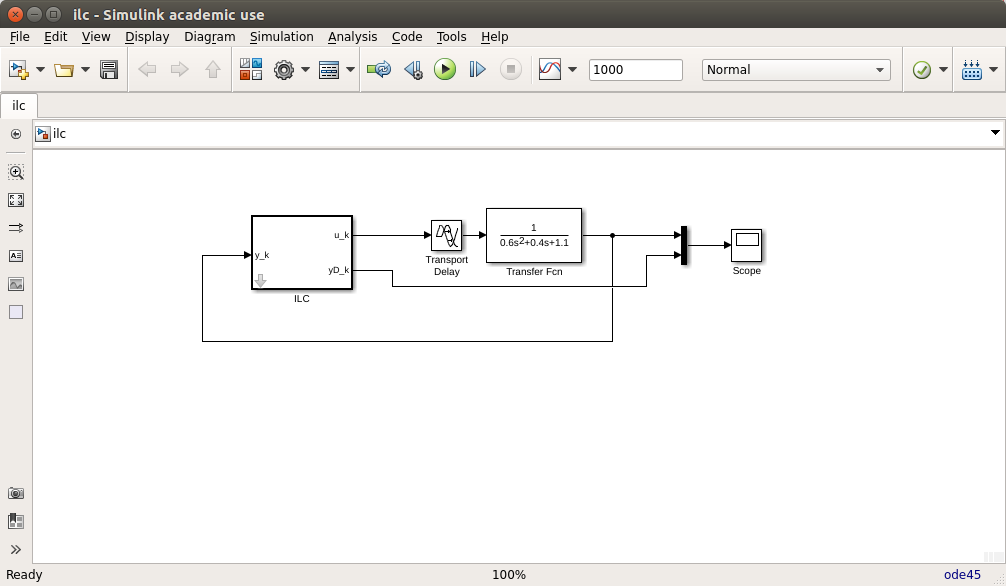
The 'Transport Delay' and 'Transfer Fcn' represent the dynamics of the system we wish to control. The ILC block attempts to learn a set of inputs to achieve a desired output sequence, by repeating the input sequence multiple times with feedback corrections due to error each time.
The fundamental update equation is u(k+N-p) = u(k-1) + g*e(k) where u is the input, k is the time step, N is the length of the repeating sequence, p is the learning offset, g is the learning rate and e(k) = yDes(k mod N) - y(k) is the error between the desired output yDes and the achieved output y. In short, the input p steps back in the sequence, next time round, is corrected using the current measured error. The initial settings are equal to the desired sequence, u(k)=yDes(k) for k=1..N, assuming that the system, perhaps with a simple controller, will already attempt to follow the input.
The file ilc.mdl (shown in image above) implements ILC for an example system with a delay, some dynamics, and a gain other that unity. The desired sequence is smooth but a bit weird, yDes(k) = sin(2pik/180)^3 for k=1..180 and time step dt=0.5s. With learning rate gamma=0.12, the output converges to the desired output as shown.
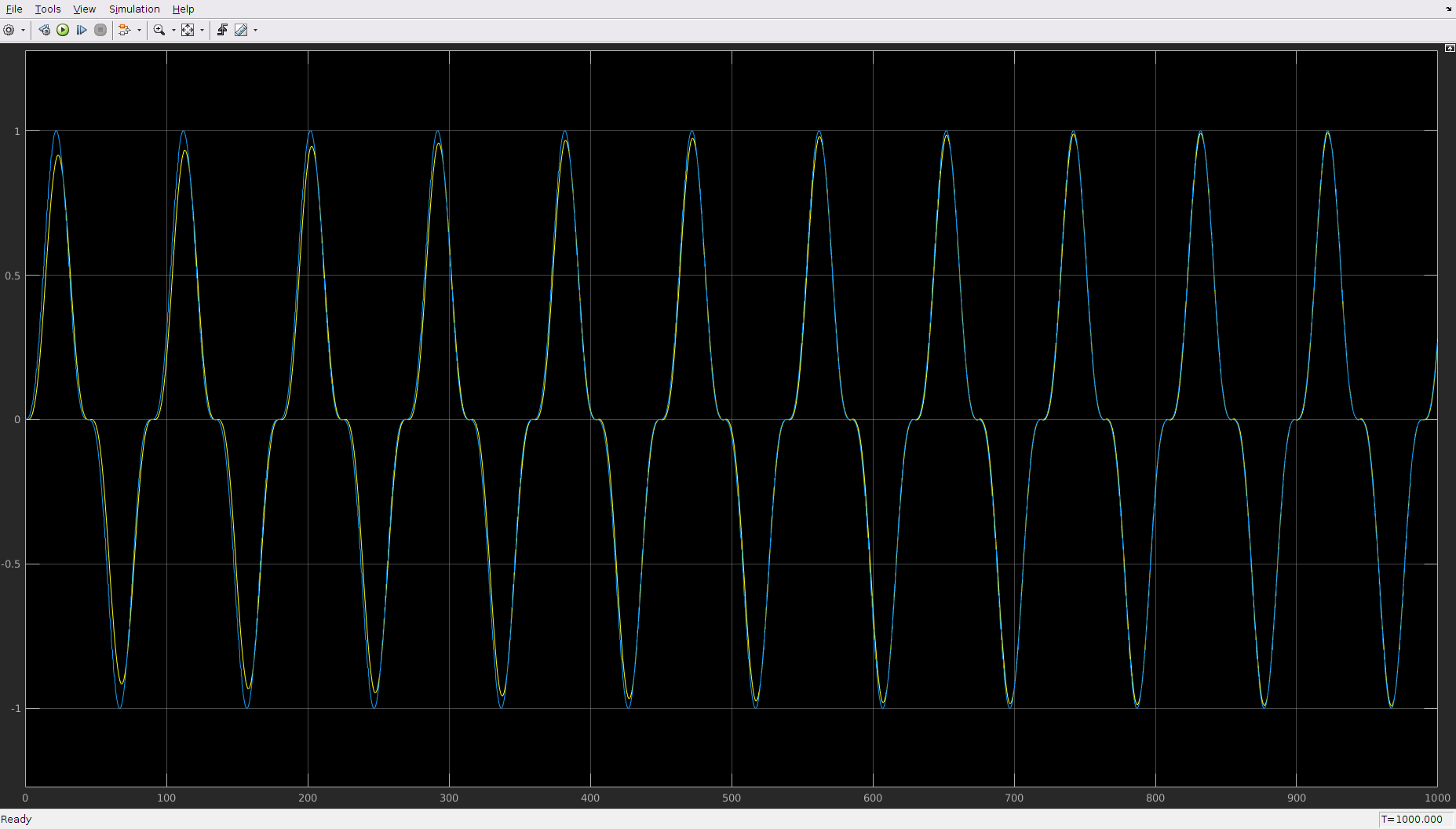
The file ilc_ramp.mdl changes the desired sequence to be a sequence of ramped steps, which is continuous but non-smooth due to the changes in gradient. Under ILC, the system makes an effort to follow the sequence, shown by the decreasing error at the step levels. However, serious ringing is seen at the corners as the simulation progresses. This needs some work: the signal is possibly too fast for the system to follow, suggesting the need to increase the time step, and perhaps smooth the corners somehow.
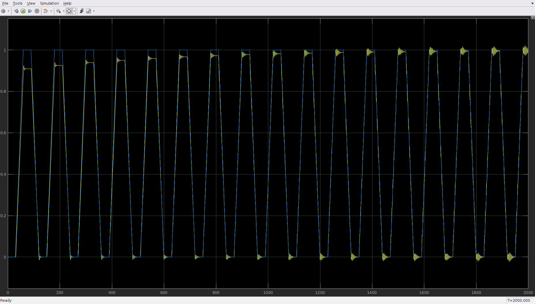
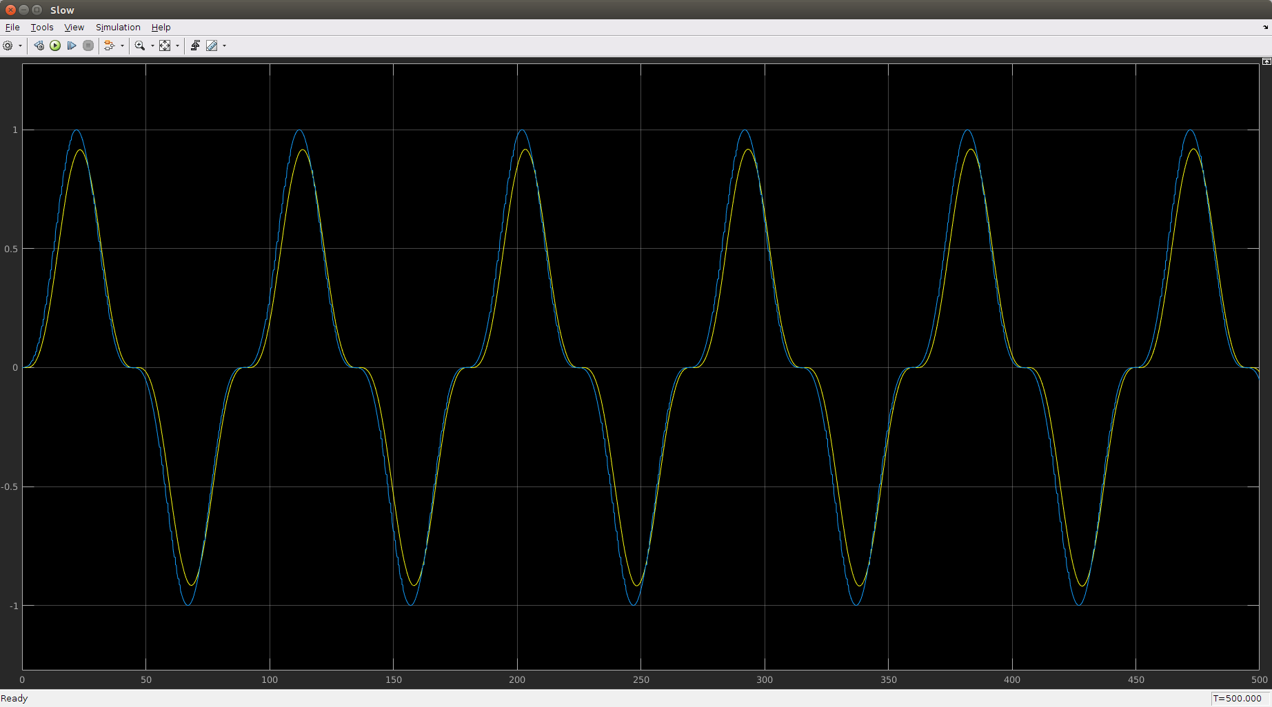
The file ilc_rate_demo.mdl replicates the basic example three times with different learning rates, giving the results shown below, each scope comparing the output with the desired output. With low gamma, the output doesn't change. With medium gamma, close inspection shows that the gap does decrease, but very slowly, and the two signals still don't match after 5 cycles of the whole sequence. With high gamma, the sequence match almost exactly after just one cycle, but by the fifth, we see signs of potential instability appearing. Hence, the learning rate must be tuned according to the familiar trade-off for any feedback gain: too low and we get sluggish performance, but too high and we get instability.
 Low gamma
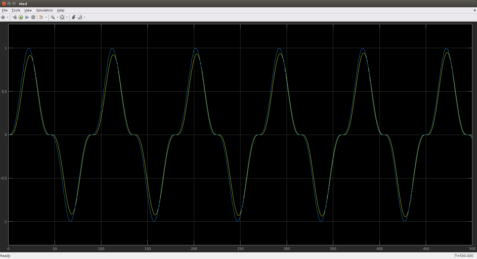 Medium gamma
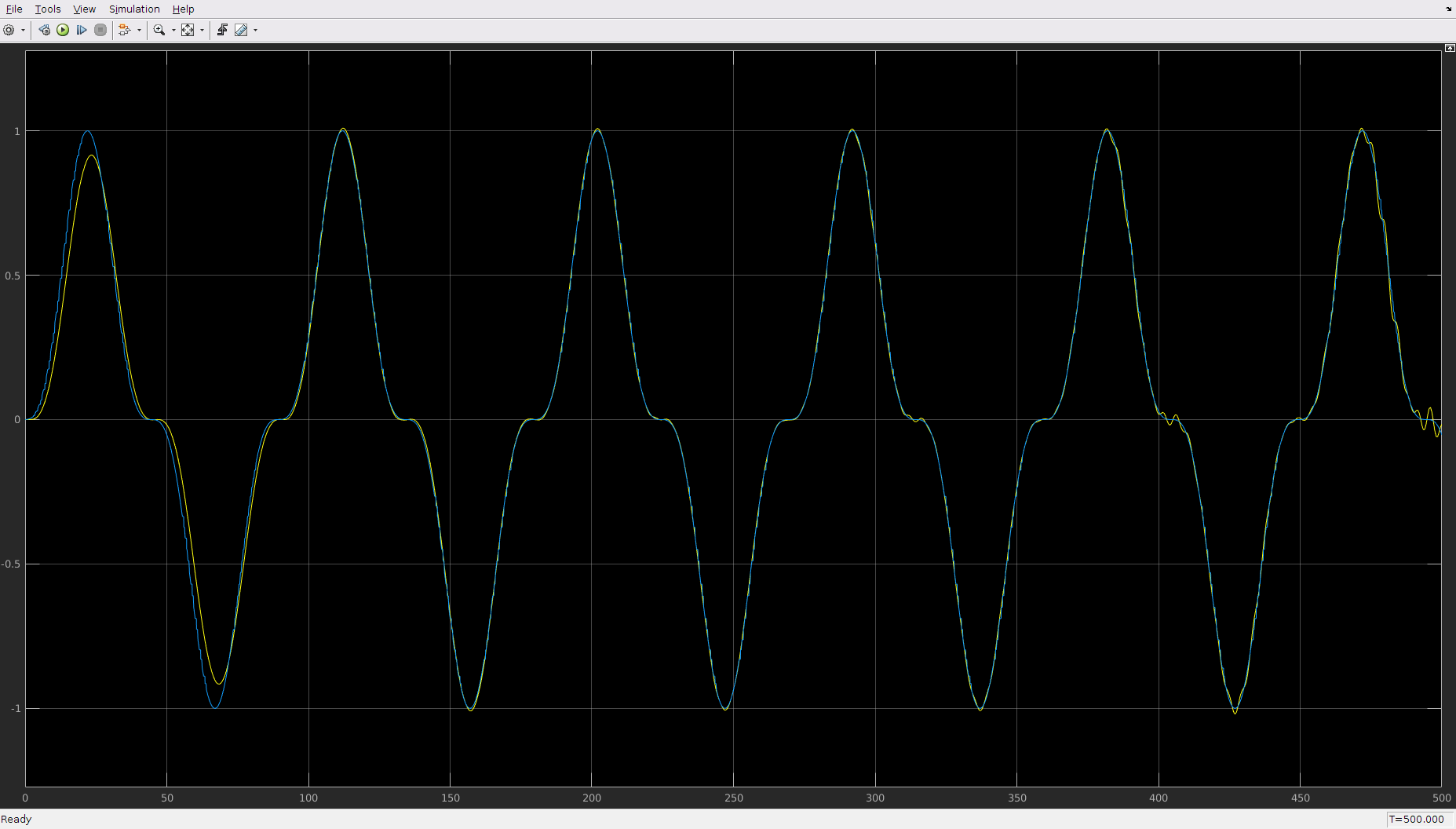 High gamma
The file ilc_drone.mdl represents one translational axis of a Parrot AR Drone, with delayed dynamics as identified by Greatwood and Richards (2019) and stabilized by a simple PD controller. This example uses a longer tracking offset, p=9, to accommodate the delay and relatively slow response of the drone.